d3-force-3d

Extended version of d3-force to support other dimensions besides 2D, via the method numDimensions, supporting the values 1, 2 or 3 (default to 2). Fully backwards compatible with d3-force (version 1.1.0), and should just work as a drop-in replacement d3 module.
This module implements a velocity Verlet numerical integrator for simulating physical forces on particles. The simulation is simplified: it assumes a constant unit time step Δt = 1 for each step, and a constant unit mass m = 1 for all particles. As a result, a force F acting on a particle is equivalent to a constant acceleration a over the time interval Δt, and can be simulated simply by adding to the particle’s velocity, which is then added to the particle’s position.
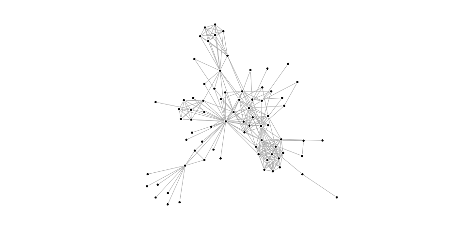
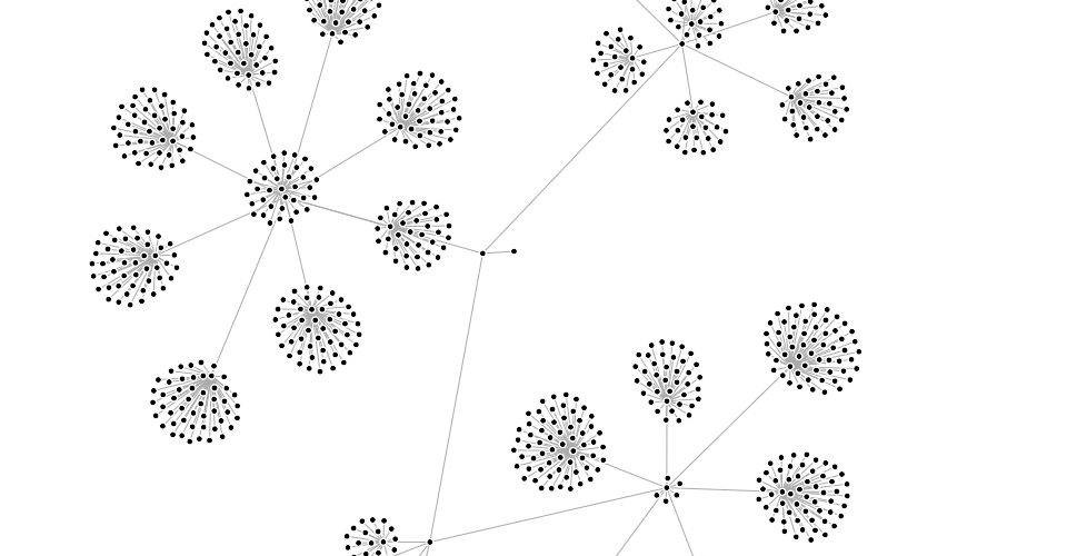
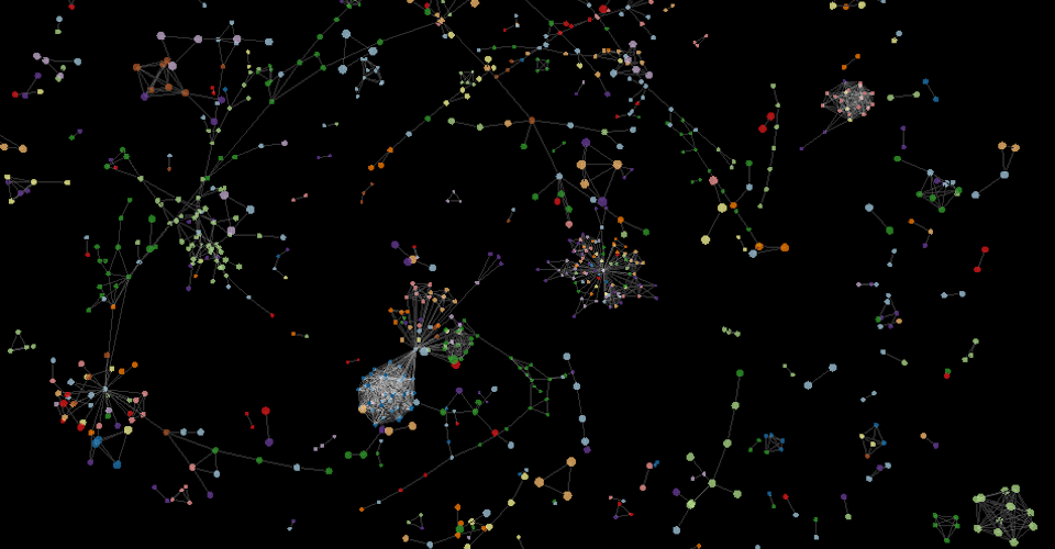
In the domain of information visualization, physical simulations are useful for studying networks and hierarchies!


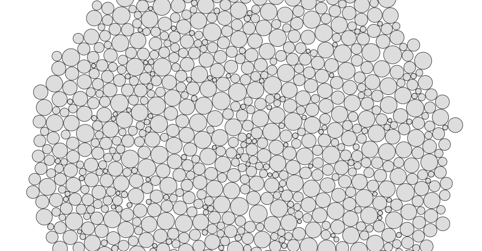
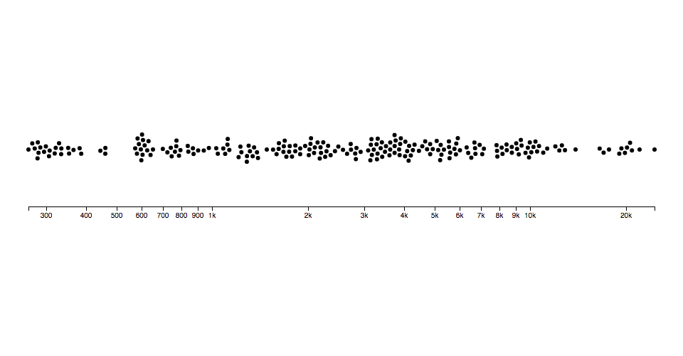
You can also simulate circles (disks) with collision, such as for bubble charts or beeswarm plots:


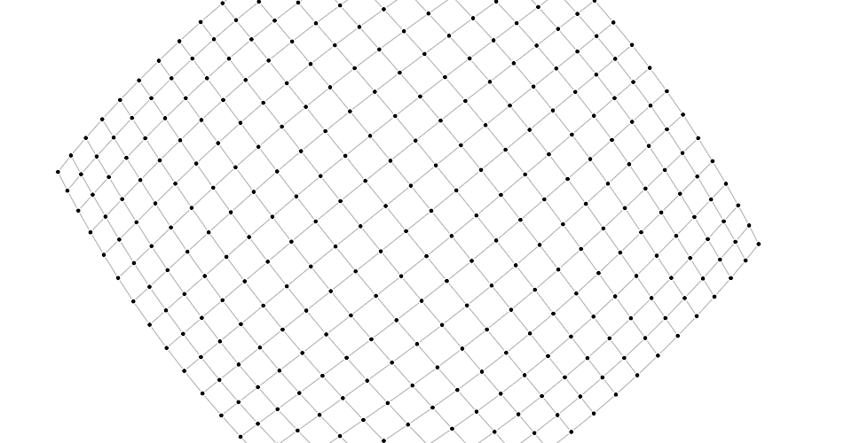
You can even use it as a rudimentary physics engine, say to simulate cloth:

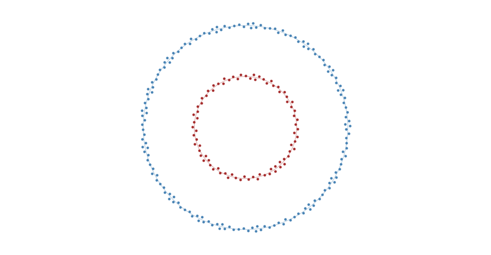
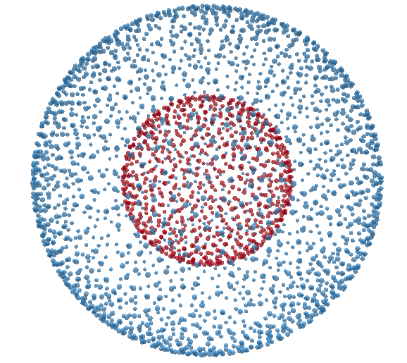
With this module update, you can also run the simulation in one, two or three dimensions:

To use this module, create a simulation for an array of nodes, and compose the desired forces. Then listen for tick events to render the nodes as they update in your preferred graphics system, such as Canvas, SVG or WebGL.
Installing
If you use NPM, npm install d3-force-3d. Otherwise, download the latest release. You can also load directly from the global npmJS registry, as a bundled standalone library. AMD, CommonJS, and vanilla environments are supported. In vanilla, a d3_force global is exported:
<script src="https://unpkg.com/d3-force-3d/build/d3-force-3d.bundle.min.js"></script>
<script>

var simulation = d3_force.forceSimulation(nodes);

</script>
Try d3-force-3d in your browser.
API Reference
Simulation
# d3.forceSimulation([nodes]) <>
Creates a new simulation with the specified array of nodes and no forces. If nodes is not specified, it defaults to the empty array. The simulator starts automatically; use simulation.on to listen for tick events as the simulation runs. If you wish to run the simulation manually instead, call simulation.stop, and then call simulation.tick as desired.
# simulation.restart() <>
Restarts the simulation’s internal timer and returns the simulation. In conjunction with simulation.alphaTarget or simulation.alpha, this method can be used to “reheat” the simulation during interaction, such as when dragging a node, or to resume the simulation after temporarily pausing it with simulation.stop.
# simulation.stop() <>
Stops the simulation’s internal timer, if it is running, and returns the simulation. If the timer is already stopped, this method does nothing. This method is useful for running the simulation manually; see simulation.tick.
# simulation.tick() <>
Increments the current alpha by (alphaTarget - alpha) × alphaDecay; then invokes each registered force, passing the new alpha; then decrements each node’s velocity by velocity × velocityDecay; lastly increments each node’s position by velocity.
This method does not dispatch events; events are only dispatched by the internal timer when the simulation is started automatically upon creation or by calling simulation.restart. The natural number of ticks when the simulation is started is ⌈log(alphaMin) / log(1 - alphaDecay)⌉; by default, this is 300.
This method can be used in conjunction with simulation.stop to compute a static force layout. For large graphs, static layouts should be computed in a web worker to avoid freezing the user interface.
# simulation.numDimensions([numDimensions]) <>
If numDimensions is specified, sets the simulation’s number of dimensions to use (1, 2 or 3), re-initializes any bound forces and returns the simulation. If numSimulations is not specified, returns the current simulation’s number of dimensions, which defaults to 2.
A one-dimensional simulation will only consider and manipulate the x and vx coordinate attributes, while a two-dimensional will extend the domain to y and vy, and a three-dimensional to z and vz.
# simulation.nodes([nodes]) <>
If nodes is specified, sets the simulation’s nodes to the specified array of objects, initializing their positions and velocities if necessary, and then re-initializes any bound forces; returns the simulation. If nodes is not specified, returns the simulation’s array of nodes as specified to the constructor.
Each node must be an object. The following properties are assigned by the simulation:
index - the node’s zero-based index into nodesx - the node’s current x-positiony - the node’s current y-position (if using 2 or more dimensions)z - the node’s current z-position (if using 3 dimensions)vx - the node’s current x-velocityvy - the node’s current y-velocity (if using 2 or more dimensions)vz - the node’s current z-velocity (if using 3 dimensions)
The position ⟨x[,y[,z]]⟩ and velocity ⟨vx[,vy[,vz]]⟩ may be subsequently modified by forces and by the simulation. If either applicable vx, vy or vz is NaN, the velocity is initialized to ⟨0,0,0⟩. If either applicable x, y or z is NaN, the 2D position is initialized in a phyllotaxis arrangement, so chosen to ensure a deterministic, uniform distribution around the origin.
To fix a node in a given position, you may specify three additional properties:
fx - the node’s fixed x-positionfy - the node’s fixed y-positionfz - the node’s fixed z-position
At the end of each tick, after the application of any forces, a node with a defined node.fx has node.x reset to this value and node.vx set to zero; likewise, in 2 dimensions or higher a node with a defined node.fy has node.y reset to this value and node.vy set to zero, and in 3-dimensions a node with a defined node.fz has node.z reset to this value and node.vz set to zero. To unfix a node that was previously fixed, set node.fx, node.fy and node.fz to null, or delete these properties.
If the specified array of nodes is modified, such as when nodes are added to or removed from the simulation, this method must be called again with the new (or changed) array to notify the simulation and bound forces of the change; the simulation does not make a defensive copy of the specified array.
# simulation.alpha([alpha]) <>
If alpha is specified, sets the current alpha to the specified number in the range [0,1] and returns this simulation. If alpha is not specified, returns the current alpha value, which defaults to 1.
# simulation.alphaMin([min]) <>
If min is specified, sets the minimum alpha to the specified number in the range [0,1] and returns this simulation. If min is not specified, returns the current minimum alpha value, which defaults to 0.001. The simulation’s internal timer stops when the current alpha is less than the minimum alpha. The default alpha decay rate of ~0.0228 corresponds to 300 iterations.
# simulation.alphaDecay([decay]) <>
If decay is specified, sets the alpha decay rate to the specified number in the range [0,1] and returns this simulation. If decay is not specified, returns the current alpha decay rate, which defaults to 0.0228… = 1 - pow(0.001, 1 / 300) where 0.001 is the default minimum alpha.
The alpha decay rate determines how quickly the current alpha interpolates towards the desired target alpha; since the default target alpha is zero, by default this controls how quickly the simulation cools. Higher decay rates cause the simulation to stabilize more quickly, but risk getting stuck in a local minimum; lower values cause the simulation to take longer to run, but typically converge on a better layout. To have the simulation run forever at the current alpha, set the decay rate to zero; alternatively, set a target alpha greater than the minimum alpha.
# simulation.alphaTarget([target]) <>
If target is specified, sets the current target alpha to the specified number in the range [0,1] and returns this simulation. If target is not specified, returns the current target alpha value, which defaults to 0.
# simulation.velocityDecay([decay]) <>
If decay is specified, sets the velocity decay factor to the specified number in the range [0,1] and returns this simulation. If decay is not specified, returns the current velocity decay factor, which defaults to 0.4. The decay factor is akin to atmospheric friction; after the application of any forces during a tick, each node’s velocity is multiplied by 1 - decay. As with lowering the alpha decay rate, less velocity decay may converge on a better solution, but risks numerical instabilities and oscillation.
# simulation.force(name[, force]) <>
If force is specified, assigns the force for the specified name and returns this simulation. If force is not specified, returns the force with the specified name, or undefined if there is no such force. (By default, new simulations have no forces.) For example, to create a new simulation to layout a graph, you might say:
var simulation = d3.forceSimulation(nodes)
    .force("charge", d3.forceManyBody())
    .force("link", d3.forceLink(links))
    .force("center", d3.forceCenter());
To remove the force with the given name, pass null as the force. For example, to remove the charge force:
simulation.force("charge", null);
# simulation.find(x[, y[, z]][, radius]) <>
Returns the node closest to the position ⟨x,y,z⟩ with the given search radius. If radius is not specified, it defaults to infinity. If there is no node within the search area, returns undefined.
# simulation.on(typenames, [listener]) <>
If listener is specified, sets the event listener for the specified typenames and returns this simulation. If an event listener was already registered for the same type and name, the existing listener is removed before the new listener is added. If listener is null, removes the current event listeners for the specified typenames, if any. If listener is not specified, returns the first currently-assigned listener matching the specified typenames, if any. When a specified event is dispatched, each listener will be invoked with the this context as the simulation.
The typenames is a string containing one or more typename separated by whitespace. Each typename is a type, optionally followed by a period (.) and a name, such as tick.foo and tick.bar; the name allows multiple listeners to be registered for the same type. The type must be one of the following:
tick - after each tick of the simulation’s internal timer.end - after the simulation’s timer stops when alpha < alphaMin.
Note that tick events are not dispatched when simulation.tick is called manually; events are only dispatched by the internal timer and are intended for interactive rendering of the simulation. To affect the simulation, register forces instead of modifying nodes’ positions or velocities inside a tick event listener.
See dispatch.on for details.
Forces
A force is simply a function that modifies nodes’ positions or velocities; in this context, a force can apply a classical physical force such as electrical charge or gravity, or it can resolve a geometric constraint, such as keeping nodes within a bounding box or keeping linked nodes a fixed distance apart. For example, a simple positioning force that moves nodes towards the origin ⟨0,0⟩ in a 2D simulation might be implemented as:
function force(alpha) {
  for (var i = 0, n = nodes.length, node, k = alpha * 0.1; i < n; ++i) {
    node = nodes[i];
    node.vx -= node.x * k;
    node.vy -= node.y * k;
  }
}
Forces typically read the node’s current position ⟨x,y,z⟩ and then add to (or subtract from) the node’s velocity ⟨vx,vy,vz⟩. However, forces may also “peek ahead” to the anticipated next position of the node, ⟨x + vx,y + vy,z + vz⟩; this is necessary for resolving geometric constraints through iterative relaxation. Forces may also modify the position directly, which is sometimes useful to avoid adding energy to the simulation, such as when recentering the simulation in the viewport.
Simulations typically compose multiple forces as desired. This module provides several for your enjoyment:
Forces may optionally implement force.initialize to receive the simulation’s array of nodes.
# force(alpha) <>
Applies this force, optionally observing the specified alpha. Typically, the force is applied to the array of nodes previously passed to force.initialize, however, some forces may apply to a subset of nodes, or behave differently. For example, d3.forceLink applies to the source and target of each link.
# force.initialize(nodes) <>
Assigns the array of nodes to this force. This method is called when a force is bound to a simulation via simulation.force and when the simulation’s nodes change via simulation.nodes. A force may perform necessary work during initialization, such as evaluating per-node parameters, to avoid repeatedly performing work during each application of the force.
Centering
The centering force translates nodes uniformly so that the mean position of all nodes (the center of mass if all nodes have equal weight) is at the given position ⟨x,y,z⟩. This force modifies the positions of nodes on each application; it does not modify velocities, as doing so would typically cause the nodes to overshoot and oscillate around the desired center. This force helps keeps nodes in the center of the viewport, and unlike the positioning force, it does not distort their relative positions.
# d3.forceCenter([x[, y[, z]]]) <>
Creates a new centering force with the specified x-, y- and z- coordinates. If x, y and z are not specified, they default to ⟨0,0,0⟩.
# center.x([x]) <>
If x is specified, sets the x-coordinate of the centering position to the specified number and returns this force. If x is not specified, returns the current x-coordinate, which defaults to zero.
# center.y([y]) <>
If y is specified, sets the y-coordinate of the centering position to the specified number and returns this force. If y is not specified, returns the current y-coordinate, which defaults to zero.
# center.z([z]) <>
If z is specified, sets the z-coordinate of the centering position to the specified number and returns this force. If z is not specified, returns the current z-coordinate, which defaults to zero.
Collision
The collision force treats nodes as lengths, circles or spheres (respectively for 1D, 2D or 3D) with a given radius, rather than points, and prevents nodes from overlapping. More formally, two nodes a and b are separated so that the distance between a and b is at least radius(a) + radius(b). To reduce jitter, this is by default a “soft” constraint with a configurable strength and iteration count.
# d3.forceCollide([radius]) <>
Creates a new circle collision force with the specified radius. If radius is not specified, it defaults to the constant one for all nodes.
# collide.radius([radius]) <>
If radius is specified, sets the radius accessor to the specified number or function, re-evaluates the radius accessor for each node, and returns this force. If radius is not specified, returns the current radius accessor, which defaults to:
function radius() {
  return 1;
}
The radius accessor is invoked for each node in the simulation, being passed the node and its zero-based index. The resulting number is then stored internally, such that the radius of each node is only recomputed when the force is initialized or when this method is called with a new radius, and not on every application of the force.
# collide.strength([strength]) <>
If strength is specified, sets the force strength to the specified number in the range [0,1] and returns this force. If strength is not specified, returns the current strength which defaults to 0.7.
Overlapping nodes are resolved through iterative relaxation. For each node, the other nodes that are anticipated to overlap at the next tick (using the anticipated positions ⟨x + vx,y + vy,z + vz⟩) are determined; the node’s velocity is then modified to push the node out of each overlapping node. The change in velocity is dampened by the force’s strength such that the resolution of simultaneous overlaps can be blended together to find a stable solution.
# collide.iterations([iterations]) <>
If iterations is specified, sets the number of iterations per application to the specified number and returns this force. If iterations is not specified, returns the current iteration count which defaults to 1. Increasing the number of iterations greatly increases the rigidity of the constraint and avoids partial overlap of nodes, but also increases the runtime cost to evaluate the force.
Links
The link force pushes linked nodes together or apart according to the desired link distance. The strength of the force is proportional to the difference between the linked nodes’ distance and the target distance, similar to a spring force.
# d3.forceLink([links]) <>
Creates a new link force with the specified links and default parameters. If links is not specified, it defaults to the empty array.
# link.links([links]) <>
If links is specified, sets the array of links associated with this force, recomputes the distance and strength parameters for each link, and returns this force. If links is not specified, returns the current array of links, which defaults to the empty array.
Each link is an object with the following properties:
source - the link’s source node; see simulation.nodestarget - the link’s target node; see simulation.nodesindex - the zero-based index into links, assigned by this method
For convenience, a link’s source and target properties may be initialized using numeric or string identifiers rather than object references; see link.id. When the link force is initialized (or re-initialized, as when the nodes or links change), any link.source or link.target property which is not an object is replaced by an object reference to the corresponding node with the given identifier.
If the specified array of links is modified, such as when links are added to or removed from the simulation, this method must be called again with the new (or changed) array to notify the force of the change; the force does not make a defensive copy of the specified array.
# link.id([id]) <>
If id is specified, sets the node id accessor to the specified function and returns this force. If id is not specified, returns the current node id accessor, which defaults to the numeric node.index:
function id(d) {
  return d.index;
}
The default id accessor allows each link’s source and target to be specified as a zero-based index into the nodes array. For example:
var nodes = [
{"id": "Alice"},
{"id": "Bob"},
{"id": "Carol"}
];
var links = [
{"source": 0, "target": 1},
{"source": 1, "target": 2}
];
Now consider a different id accessor that returns a string:
function id(d) {
  return d.id;
}
With this accessor, you can use named sources and targets:
var nodes = [
  {"id": "Alice"},
  {"id": "Bob"},
  {"id": "Carol"}
];

var links = [
  {"source": "Alice", "target": "Bob"},
  {"source": "Bob", "target": "Carol"}
];
This is particularly useful when representing graphs in JSON, as JSON does not allow references. See this example.
The id accessor is invoked for each node whenever the force is initialized, as when the nodes or links change, being passed the node and its zero-based index.
# link.distance([distance]) <>
If distance is specified, sets the distance accessor to the specified number or function, re-evaluates the distance accessor for each link, and returns this force. If distance is not specified, returns the current distance accessor, which defaults to:
function distance() {
  return 30;
}
The distance accessor is invoked for each link, being passed the link and its zero-based index. The resulting number is then stored internally, such that the distance of each link is only recomputed when the force is initialized or when this method is called with a new distance, and not on every application of the force.
# link.strength([strength]) <>
If strength is specified, sets the strength accessor to the specified number or function, re-evaluates the strength accessor for each link, and returns this force. If strength is not specified, returns the current strength accessor, which defaults to:
function strength(link) {
  return 1 / Math.min(count(link.source), count(link.target));
}
Where count(node) is a function that returns the number of links with the given node as a source or target. This default was chosen because it automatically reduces the strength of links connected to heavily-connected nodes, improving stability.
The strength accessor is invoked for each link, being passed the link and its zero-based index. The resulting number is then stored internally, such that the strength of each link is only recomputed when the force is initialized or when this method is called with a new strength, and not on every application of the force.
# link.iterations([iterations]) <>
If iterations is specified, sets the number of iterations per application to the specified number and returns this force. If iterations is not specified, returns the current iteration count which defaults to 1. Increasing the number of iterations greatly increases the rigidity of the constraint and is useful for complex structures such as lattices, but also increases the runtime cost to evaluate the force.
Many-Body
The many-body (or n-body) force applies mutually amongst all nodes. It can be used to simulate gravity (attraction) if the strength is positive, or electrostatic charge (repulsion) if the strength is negative. This implementation uses binary-, quad-, or oct-trees (1D, 2D or 3D respectively) and the Barnes–Hut approximation to greatly improve performance; the accuracy can be customized using the theta parameter.
Unlike links, which only affect two linked nodes, the charge force is global: every node affects every other node, even if they are on disconnected subgraphs.
# d3.forceManyBody() <>
Creates a new many-body force with the default parameters.
# manyBody.strength([strength]) <>
If strength is specified, sets the strength accessor to the specified number or function, re-evaluates the strength accessor for each node, and returns this force. A positive value causes nodes to attract each other, similar to gravity, while a negative value causes nodes to repel each other, similar to electrostatic charge. If strength is not specified, returns the current strength accessor, which defaults to:
function strength() {
  return -30;
}
The strength accessor is invoked for each node in the simulation, being passed the node and its zero-based index. The resulting number is then stored internally, such that the strength of each node is only recomputed when the force is initialized or when this method is called with a new strength, and not on every application of the force.
# manyBody.theta([theta]) <>
If theta is specified, sets the Barnes–Hut approximation criterion to the specified number and returns this force. If theta is not specified, returns the current value, which defaults to 0.9.
To accelerate computation, this force implements the Barnes–Hut approximation which takes O(n log n) per application where n is the number of nodes. For each application, a binarytree, quadtree or octree stores the current node positions; then for each node, the combined force of all other nodes on the given node is computed. For a cluster of nodes that is far away, the charge force can be approximated by treating the cluster as a single, larger node. The theta parameter determines the accuracy of the approximation: if the ratio w / l of the width w of the tree cell to the distance l from the node to the cell’s center of mass is less than theta, all nodes in the given cell are treated as a single node rather than individually.
# manyBody.distanceMin([distance]) <>
If distance is specified, sets the minimum distance between nodes over which this force is considered. If distance is not specified, returns the current minimum distance, which defaults to 1. A minimum distance establishes an upper bound on the strength of the force between two nearby nodes, avoiding instability. In particular, it avoids an infinitely-strong force if two nodes are exactly coincident; in this case, the direction of the force is random.
# manyBody.distanceMax([distance]) <>
If distance is specified, sets the maximum distance between nodes over which this force is considered. If distance is not specified, returns the current maximum distance, which defaults to infinity. Specifying a finite maximum distance improves performance and produces a more localized layout.
Positioning
The x-, y- and z-positioning forces push nodes towards a desired position along the given dimension with a configurable strength. The radial force is similar, except it pushes nodes towards the closest point on a given circle/sphere. The strength of the force is proportional to the one-dimensional distance between the node’s position and the target position. While these forces can be used to position individual nodes, they are intended primarily for global forces that apply to all (or most) nodes.
# d3.forceX([x]) <>
Creates a new positioning force along the x-axis towards the given position x. If x is not specified, it defaults to 0.
# x.strength([strength]) <>
If strength is specified, sets the strength accessor to the specified number or function, re-evaluates the strength accessor for each node, and returns this force. The strength determines how much to increment the node’s x-velocity: (x - node.x) × strength. For example, a value of 0.1 indicates that the node should move a tenth of the way from its current x-position to the target x-position with each application. Higher values moves nodes more quickly to the target position, often at the expense of other forces or constraints. A value outside the range [0,1] is not recommended.
If strength is not specified, returns the current strength accessor, which defaults to:
function strength() {
  return 0.1;
}
The strength accessor is invoked for each node in the simulation, being passed the node and its zero-based index. The resulting number is then stored internally, such that the strength of each node is only recomputed when the force is initialized or when this method is called with a new strength, and not on every application of the force.
# x.x([x]) <>
If x is specified, sets the x-coordinate accessor to the specified number or function, re-evaluates the x-accessor for each node, and returns this force. If x is not specified, returns the current x-accessor, which defaults to:
function x() {
  return 0;
}
The x-accessor is invoked for each node in the simulation, being passed the node and its zero-based index. The resulting number is then stored internally, such that the target x-coordinate of each node is only recomputed when the force is initialized or when this method is called with a new x, and not on every application of the force.
# d3.forceY([y]) <>
Creates a new positioning force along the y-axis towards the given position y. If y is not specified, it defaults to 0.
# y.strength([strength]) <>
If strength is specified, sets the strength accessor to the specified number or function, re-evaluates the strength accessor for each node, and returns this force. The strength determines how much to increment the node’s y-velocity: (y - node.y) × strength. For example, a value of 0.1 indicates that the node should move a tenth of the way from its current y-position to the target y-position with each application. Higher values moves nodes more quickly to the target position, often at the expense of other forces or constraints. A value outside the range [0,1] is not recommended.
If strength is not specified, returns the current strength accessor, which defaults to:
function strength() {
  return 0.1;
}
The strength accessor is invoked for each node in the simulation, being passed the node and its zero-based index. The resulting number is then stored internally, such that the strength of each node is only recomputed when the force is initialized or when this method is called with a new strength, and not on every application of the force.
# y.y([y]) <>
If y is specified, sets the y-coordinate accessor to the specified number or function, re-evaluates the y-accessor for each node, and returns this force. If y is not specified, returns the current y-accessor, which defaults to:
function y() {
  return 0;
}
The y-accessor is invoked for each node in the simulation, being passed the node and its zero-based index. The resulting number is then stored internally, such that the target y-coordinate of each node is only recomputed when the force is initialized or when this method is called with a new y, and not on every application of the force.
# d3.forceZ([z]) <>
Creates a new positioning force along the z-axis towards the given position z. If z is not specified, it defaults to 0.
# z.strength([strength]) <>
If strength is specified, sets the strength accessor to the specified number or function, re-evaluates the strength accessor for each node, and returns this force. The strength determines how much to increment the node’s z-velocity: (z - node.z) × strength. For example, a value of 0.1 indicates that the node should move a tenth of the way from its current z-position to the target z-position with each application. Higher values moves nodes more quickly to the target position, often at the expense of other forces or constraints. A value outside the range [0,1] is not recommended.
If strength is not specified, returns the current strength accessor, which defaults to:
function strength() {
  return 0.1;
}
The strength accessor is invoked for each node in the simulation, being passed the node and its zero-based index. The resulting number is then stored internally, such that the strength of each node is only recomputed when the force is initialized or when this method is called with a new strength, and not on every application of the force.
# z.z([z]) <>
If z is specified, sets the z-coordinate accessor to the specified number or function, re-evaluates the z-accessor for each node, and returns this force. If z is not specified, returns the current z-accessor, which defaults to:
function z() {
  return 0;
}
The z-accessor is invoked for each node in the simulation, being passed the node and its zero-based index. The resulting number is then stored internally, such that the target z-coordinate of each node is only recomputed when the force is initialized or when this method is called with a new z, and not on every application of the force.
# d3.forceRadial(radius[, x][, y][, z]) <>


Creates a new positioning force towards a circle or sphere of the specified radius centered at ⟨x,y,z⟩. If x, y and z are not specified, they default to ⟨0,0,0⟩.
# radial.strength([strength]) <>
If strength is specified, sets the strength accessor to the specified number or function, re-evaluates the strength accessor for each node, and returns this force. The strength determines how much to increment the node’s x-, y and z-velocity. For example, a value of 0.1 indicates that the node should move a tenth of the way from its current position to the closest point on the sphere perimeter with each application. Higher values moves nodes more quickly to the target position, often at the expense of other forces or constraints. A value outside the range [0,1] is not recommended.
If strength is not specified, returns the current strength accessor, which defaults to:
function strength() {

  return 0.1;

}
The strength accessor is invoked for each node in the simulation, being passed the node and its zero-based index. The resulting number is then stored internally, such that the strength of each node is only recomputed when the force is initialized or when this method is called with a new strength, and not on every application of the force.
# radial.radius([radius]) <>
If radius is specified, sets the circle radius to the specified number or function, re-evaluates the radius accessor for each node, and returns this force. If radius is not specified, returns the current radius accessor.
The radius accessor is invoked for each node in the simulation, being passed the node and its zero-based index. The resulting number is then stored internally, such that the target radius of each node is only recomputed when the force is initialized or when this method is called with a new radius, and not on every application of the force.
# radial.x([x]) <>
If x is specified, sets the x-coordinate of the sphere center to the specified number and returns this force. If x is not specified, returns the current x-coordinate of the center, which defaults to zero.
# radial.y([y]) <>
If y is specified, sets the y-coordinate of the sphere center to the specified number and returns this force. If y is not specified, returns the current y-coordinate of the center, which defaults to zero.
# radial.z([z]) <>
If z is specified, sets the z-coordinate of the sphere center to the specified number and returns this force. If z is not specified, returns the current z-coordinate of the center, which defaults to zero.


