pyrsgis

Python-for-Remote-Sensing-and-GIS

pyrsgis enables the user to read, process and export GeoTIFFs. The module is built on the GDAL library but is much more convenient when it comes to reading and exporting GeoTIFs. There are several other functions available in this package that ease raster pre-processing. Please check the documentation page for a list of functions that pyrsgis offers along with the sample code.

Feedback and doubts from users are most welcome. Since this is an open-source volunatry project, I always look forward to contributors. You can write to me at [e-mail].

pyrsgis is available on both, PyPI and Anaconda. Please check the installation page for details.

Recommended citation:
Tripathy, P. pyrsgis: A Python package for remote sensing and GIS data processing. V0.4. Available at https://github.com/PratyushTripathy/pyrsgis.

Sample code (click to expand)

1. Reading .tif extension file

Import the module and define the input file path.

from pyrsgis import raster

file_path = r'D:/your_file_name.tif'

• To read all the bands of a stacked satellite image:
  

ds, arr = raster.read(file_path, bands='all')

where, ds is the data source similar to GDAL and arr is the numpy array that contains all the bands of the input raster. The arr can be 2D or 3D depending on the input data. One can check the shape of the array using the print(arr.shape) command. The bands argument in the raster.read function defaults to 'all'.

• To read a list of bands of a stacked satellite image:
  

ds, arr = raster.read(file_path, bands=[2, 3, 4])

Passing the band numbers in a list returns bands 2, 3 & 4 as three-dimensional numpy array.

• To read a specific band from stacked satellite image:
  

ds, arr = raster.read(file_path, bands=2)

Passing a single band number returns that particular band as two-dimensional numpy array.

• To read a single band TIF file:
  

ds, arr = raster.read(file_path)

Since the bands argument defaults to 'all', this will read all the bands in the input file, here, one band only.

2. Exporting .tif extension file

In all the below examples, it is assumed that the number of rows and columns, and the cell size of the input and output rasters are the same. All these are stored in the `ds` variable, please see details here: link.

• To export all bands of a 3D array:
  

out_file_path = r'D:/sample_file_all_bands.tif'
raster.export(arr, ds, out_file_path, dtype='int', bands='all')

The dtype argument in the above function by default is set to 'default', which is 'int'--16-bit integer. If the data type in the provided ds is not int and the paramter is set to default, then the data type of the ds will be used. If there is a disagreement and the dtype argument is explicitly specified, it will override the data type of ds. Please be careful to change this while exporting arrays with large values. Similarly, to export float type array (eg. NDVI), use dtype = 'float'. Data type of high pixel-depth, e.g. Integer32, Integer64, or float type uses more space on hard drive, so the default has been set to integer. To export any float datatype, the argument should be passed explicitly.
These are the options for the dtype argument: byte, cfloat32, cfloat64, cint16, cint32, float32, float64, int16, int32, uint8, uint16, uint32.
The NoData value can be explicitly defined using the nodata parameter, this defaults to -9999.

• To export a list of bands of a 3D array:
  

out_file_path = r'D:/sample_file_bands_234.tif'
raster.export(arr, ds, out_file_path, bands=[2, 3, 4])

• To export any one band of a 3D array:
  

out_file_path = r'D:/sample_file_band_3.tif'
raster.export(arr, ds, out_file_path, bands=3)

• To export a single band array:
  

out_file_path = r'D:/sample_file.tif'
raster.export(arr, ds, out_file_path)

where, arr should be a 2D array.

• Export the raster with compression:
  Compression type can also be defined while exporting the raster by using the compress parameter. LZW. DEFLATE, etc. are a couple of options. Defaults to None.
  

• Example with all default parameters:
  

out_file_path = r'D:/sample_file.tif'
raster.export(band, ds, filename='pyrsgis_outFile.tif', dtype='int', bands=1, nodata=-9999, compress=None)

3. Converting TIF to CSV

GeoTIFF files can be converted to CSV files using *pyrsgis*. Every band is flattened to a single-dimensional array, and converted to CSV. These are very useful for statistical analysis.
Import the function:

from pyrsgis.convert import rastertocsv

To convert all the bands present in a folder:

your_dir = r"D:/your_raster_directory"
out_file_path = r"D:/yourFilename.csv"

rastertocsv(your_dir, filename=out_file_path)

Generally the NoData or NULL values in the raster become random negative values, negatives can be removed using the negative argument:

rastertocsv(your_dir, filename=out_file_path, negative=False)

At times the NoData or NULL values in raster become '127' or '65536', they can also be removed by declaring explicitly.

rastertocsv(your_dir, filename=out_file_path, remove=[127, 65536])

This is a trial and check process, please check the generated CSV file for such issues and handle as required.

Similarly, there are bad rows in the CSV file, representing zero value in all the bands. This takes a lot of unnecessary space on drive, it can be eliminated using:

rastertocsv(your_dir, filename=out_file_path, badrows=False)

4. Creating northing and easting using a reference raster

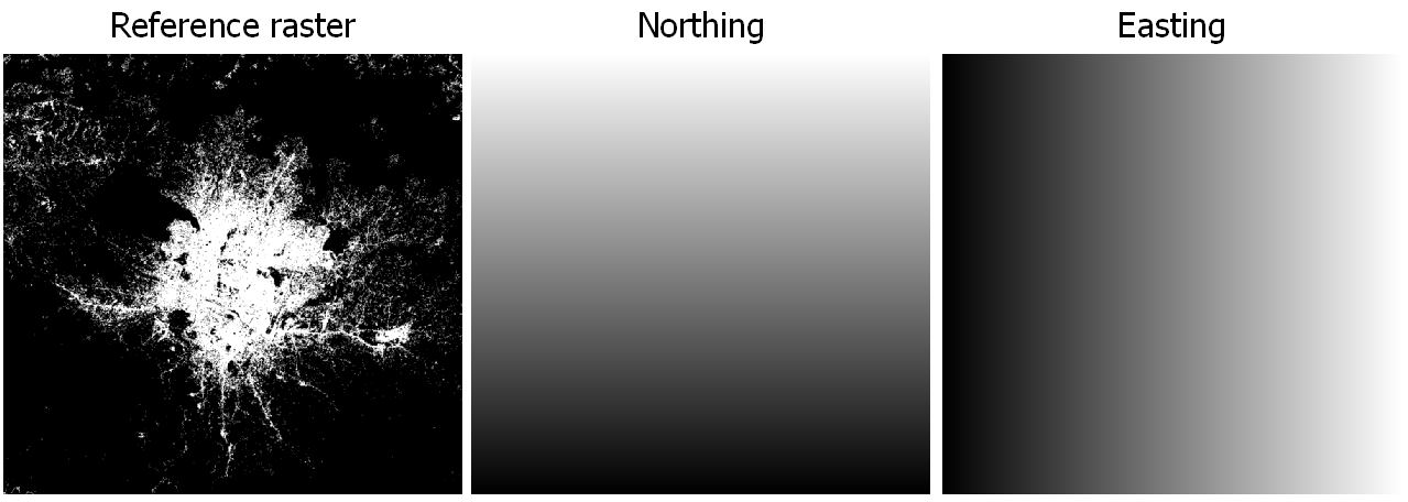
pyrsgis allows to quickly create the northing and easting rasters using a reference raster, as shown below:

The cell value in the generated rasters are the row and column number of the cell. To generate these GeoTIFF files, start by importing the function:

from pyrsgis.raster import northing, easting

reference_file_path = r'D:/your_reference_raster.tif'

northing(reference_file_path, outFile= r'D:/pyrsgis_northing.tif', flip=True)
easting(reference_file_path, outFile= r'D:/pyrsgis_easting.tif', flip=False)

As the name suggests, the flip argument flips the resulting rasters.
The value argument defaults to number. It can be changed to normalised to get a normalised layer. The other option for value argument is coordinates, which produces the raster layer with cell centroids. Please note that if the value argument is set to normalised, it will automatically adjust the flip value, i.e. False, both in easting and northing functions. Similarly, the dtype parameter auto-adjusts with the data type, but can be changed to a higher pixel depth when value argument is number. Example with all parameters:

northing(reference_file_path, outFile='pyrsgis_northing.tif', flip=True, value='number', dtype='int16')
easting(reference_file_path, outFile='pyrsgis_easting.tif', flip=False, value='number', dtype='int16')

5. Shifting raster layers

You can shift the raster layers using either the 'shift' or 'shift_file' function. The 'shift' function allows to shift the raster in the backend, whereas, the 'shift_file' directly shifts the GeoTIF file and stores another file.

To shift in the backend:

from pyrsgis import raster

# Define the path to the input file and get the data source
infile = r"D:/path_to_your_file/input.tif"
ds, arr = raster.read(infile)

# Define the amount of shift required
delta_x = 15
delta_y = 11.7

# shift the raster
shifted_ds = raster.shift(ds, x=delta_x, y=delta_y, shift_type)

# if you wish to export
raster.export(arr, ds, out_file, dtype='int', bands=1, nodata=-9999)

Here, 'ds' is the data source object that is created when the raster is read using 'raster.read' command. 'x' and 'y' are the distance for shifting the raster. The 'shift_type' command let's you move the raster either by the raster units or number of cells, the valid options are 'unit' and 'cell'. By default, the 'shift_type' is 'unit'.

To shift a GeoTIFF file:

from pyrsgis import raster

# Define the path to the input and output file
infile = r"D:/path_to_your_file/input.tif"
outfile = r"D:/path_to_your_file/shifted_output.tif"

# Define the amount of shift required
delta_x = 15
delta_y = 11.7

# shift the raster
raster.shift_file(infile, x=delta_x, y=delta_y, outfile=outfile, shift_type='unit', dtype='uint16')

Most of the parameters are same as the 'shift' function. The 'dtype' parameter is same as used in the 'raster.export' function.

6. Create image chips for Convolutional Neural Network (CNN)

CNNs require image chips for training and prediction. Remote sensing images are large sized two or three-dimesional images, this module enables creating image chips directly from TIF files or arrays. The input data and size of image chips are required.

To create image chips from array:

from pyrsgis import raster
from pyrsgis.ml import imageChipsFromArray

# read the TIF file(s) (both are of different sizes - for demonstration)
single_band_file = r'path/to/single_band.tif'
multi_band_file = r'path/to/multi_band.tif' # this is a Landsat 5 TM image (7 bands stacked)

# read the files as array using pyrsgis raster.read module
_, single_band_array = raster.read(single_band_file)
_, multi_band_array = raster.read(multi_band_file)

# create image chips
single_band_chips = imageChipsFromArray(single_band_array, x_size=5, y_size=5))
multi_band_chips = imageChipsFromArray(multi_band_array, x_size=5, y_size=5))

print(single_band_chips.shape)
print(multi_band_chips.shape)

The output:

(91125, 5, 5)
(987552, 5, 5, 7)

Image chips can also be generated directly from TIF files using following:

from pyrsgis.ml import imageChipsFromFile

# read the TIF file(s) (both are of different sizes - for demonstration)
single_band_file = r'path/to/single_band.tif'
multi_band_file = r'path/to/multi_band.tif' # this is a Landsat 5 TM image (7 bands stacked)

# create image chips
single_band_chips = imageChipsFromFile(single_band_file, x_size=5, y_size=5))
multi_band_chips = imageChipsFromFile(multi_band_file, x_size=5, y_size=5))

print(single_band_chips.shape)
print(multi_band_chips.shape)

This will result in the same output as the one above.

7. Reading directly from .tar.gz files (beta)

Currently, only Landsat data is supported.

import pyrsgis

file_path = r'D:/your_file_name.tar.gz'
your_data = pyrsgis.readtar(file_path)

The above code reads the data and stores in the your_data variable.

Various properties of the raster can be assessed using the following code:

print(your_data.rows)
print(your_data.cols)

This will display the number of rows and columns of the input data.

Similarly, the number of bands can be checked using:

print(your_data.nbands)

On reading the .tar.gz files directly, pyrsgis determines the satellite sensor. This can be checked using:

print(your_data.satellite)

This will display the satellite sensor, for instance, Landsat-5, Landsat-8, etc.

If the above code shows the correct satellite sensor, then the list of band names of the sensor (in order) can easily be checked using:

print(your_data.bandIndex)

Any particular band can be extarcted using:

band_number = 1
your_band = your_data.getband(band_number)

The above code returns the band as array which can be visualised using:

display(your_band, maptitle='Title of your image', cmap='PRGn')

or, directly using:

band_number = 1
display(your_data.getband(band_number), maptitle='Title of your image', cmap='PRGn')

The generated map can directly be saved as an image.

The extracted band can be exported using:

out_file_path = r'D:/sample_output.tif'
your_data.export(your_band, out_file_path)

This saves the extracted band to the same directory.

To export the float type raster, please define the datatype explicitly, default is 'int':

your_data.export(your_band, out_file_path, datatype='float')

The NDVI (Normalised Difference Vegetaton Index) can be computed easily.

your_ndvi = your_data.ndvi()

Normalised difference index between any two bands can be computed using:

norm_diff = your_data.nordif(bandNumber2, bandNumber1)

This computes (band2-band1)/(band2+band1) in the back end and returns a numpy array. The resulting array can be exported using:

out_file_path = r'D:/your_ndvi.tif'
your_data.export(your_ndvi, out_file_path, datatype='float')

Be careful with the float type of NDVI.