memory-graph

Installation

Install (or upgrade) memory_graph using pip:

pip install --upgrade memory_graph

Additionally Graphviz needs to be installed.

Highlights

Run a live demo in the 👉 Memory Graph Web Debugger 👈 now, no installation required!

• learn the right mental model to think about Python data (references, mutability, shallow vs deep copy)
• visualize the structure of your data to easily understand and debug any data structure
• understand function calls, variable scope, and the complete program state through call stack visualization

An example Binary Tree data structure: Or see it in the Memory Grah Web Debugger.

Videos

Quick Intro (3:49)	Mutability (17:29)

Memory Graph

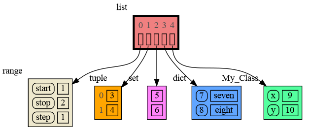
For program understanding and debugging, the memory_graph package can visualize your data, supporting many different data types, including but not limited to:

import memory_graph as mg

class My_Class:

    def __init__(self, x, y):
        self.x = x
        self.y = y

data = [ range(1, 2), (3, 4), {5, 6}, {7:'seven', 8:'eight'},  My_Class(9, 10) ]
mg.show(data)

Instead of showing the graph on screen you can also render it to an output file (see Graphviz Output Formats) using for example:

mg.render(data, "my_graph.pdf")
mg.render(data, "my_graph.svg")
mg.render(data, "my_graph.png")
mg.render(data, "my_graph.gv") # Graphviz DOT file
mg.render(data) # renders to default: 'memory_graph.pdf'

Sharing Values

In Python, assigning a list from variable a to variable b causes both variables to reference the same list value and thus share it. Consequently, any change applied through one variable will impact the other. This behavior can lead to elusive bugs if a programmer incorrectly assumes that list a and b are independent.

import memory_graph as mg # create the lists 'a' and 'b' a = [4, 3, 2] b = a b.append(1) # changing 'b' changes 'a' # print the 'a' and 'b' list print('a:', a) print('b:', b) # check if 'a' and 'b' share values print('ids:', id(a), id(b)) print('identical?:', a is b) # show all local variables in a graph mg.show( locals() )

a graph showing a and b share values

The fact that a and b share values can not be verified by printing the lists. It can be verified by comparing the identity of both variables using the id() function or by using the is comparison operator as shown in the program output below, but this quickly becomes impractical for larger programs.

a: 4, 3, 2, 1
b: 4, 3, 2, 1
ids: 126432214913216 126432214913216
identical?: True

A better way to understand what values are shared is to draw a graph using memory_graph.

Topics

Python Data Model

Call Stack

Data Model Exercises

Block

Debugging

Data Structure Examples

Sorting Algorithms

Bitwise Operators

Sliding Puzzle Solver

Configuration

Introspection

Graph Depth

Extensions

Memory Graph Web Debugger

Jupyter Notebook

ipython

Google Colab

Marimo

Animated GIF

Troubleshooting

Other Packages

Author

Bas Terwijn

Inspiration

Inspired by Python Tutor.

The main difference are that running memory_graph locally is a key design choice to support Python Tutor’s unsupported features and mirroring the data’s hierarchy improves graph readability.

Social Media

• LinkedIn
• Reddit

Supported by

Python Data Model

Learn the right mental model to think about Python data. The Python Data Model makes a distiction between immutable and mutable types:

• immutable: bool, int, float, complex, str, tuple, bytes, frozenset
• mutable: list, set, dict, classes, ... (most other types)

Immutable Type

In the code below variable a and b both reference the same tuple value (4, 3, 2). A tuple is an immutable type and therefore when we change variable b its value cannot be mutated in place, and thus an automatic copy is made and a and b each reference their own value afterwards.

import memory_graph as mg

a = (4, 3, 2)
b = a
mg.render(locals(), 'immutable1.png')

b += (1,)
mg.render(locals(), 'immutable2.png')

immutable1.png	immutable2.png

Mutable Type

With mutable types the result is different. In the code below variable a and b both reference the same list value [4, 3, 2]. A list is a mutable type and therefore when we change variable b its value can be mutated in place and thus a and b both reference the same new value afterwards. Thus changing b also changes a and vice versa. Sometimes we want this but other times we don't and then we will have to make a copy ourselfs so that a and b are independent.

import memory_graph as mg

a = [4, 3, 2]
b = a
mg.render(locals(), 'mutable1.png')

b += [1]  # equivalent to:  b.append(1)
mg.render(locals(), 'mutable2.png')

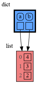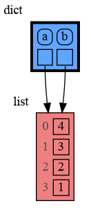mutable1.png	mutable2.png

One practical reason why Python makes the distinction between mutable and immutable types is that a value of a mutable type can be large, making it inefficient to copy each time we change it. Values of immutable type generally don't need to change as much, or are small, making copying less of a concern.

Copying Values of Mutable Type

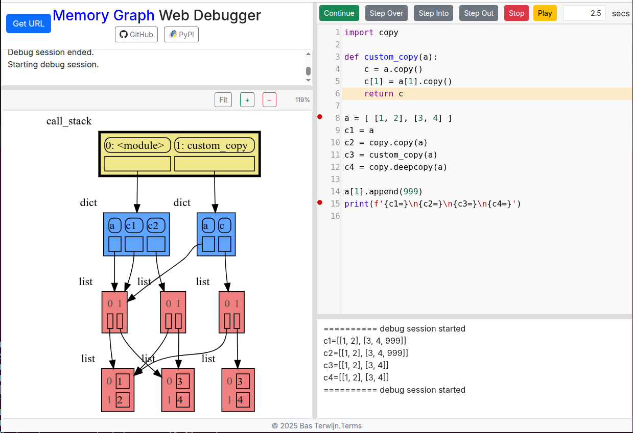
Python offers three different "copy" options that we will demonstrate using a nested list:

import memory_graph as mg
import copy

a = [ [1, 2], ['x', 'y'] ]  # a nested list (a list containing lists)

# three different ways to make a "copy" of 'a':
c1 = a
c2 = copy.copy(a)  # for list equivalent to:  a.copy() a[:] list(a)
c3 = copy.deepcopy(a)

mg.show(locals())

• c1 is an assignment, nothing is copied, all the values are shared
• c2 is a shallow copy, only the first value is copied, all the underlying values are shared
• c3 is a deep copy, all the values are copied, nothing is shared

Or see it in the Memory Grah Web Debugger.

Custom Copy

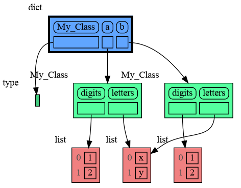
We can write our own custom copy function or method in case the three standard "copy" options don't do what we want. For example, in the code below the custom_copy() method of My_Class copies the digits but shares the letters between two objects.

import memory_graph as mg
import copy

class My_Class:

    def __init__(self):
        self.digits = [1, 2]
        self.letters = ['x', 'y']

    def custom_copy(self): 
        """ Copies 'digits' but shares 'letters'. """
        c = copy.copy(self)
        c.digits = copy.copy(self.digits)
        return c

a = My_Class()
b = a.custom_copy()

mg.show(locals())

Or see it in the Memory Grah Web Debugger.

Name Rebinding

When a and b share a mutable value, then changing the value of b changes the value of a and vice versa. However, reassigning b does not change a. When you reassign b, you only rebind the name b to another value without affecting any other variable.

import memory_graph as mg

a = [4, 3, 2]
b = a
mg.render(locals(), 'rebinding1.png')

b += [1]        # changes the value of 'b' and 'a'
b = [100, 200]  # rebinds 'b' to another value, 'a' is unaffected
mg.render(locals(), 'rebinding2.png')

rebinding1.png	rebinding2.png

Or see it in the Memory Grah Web Debugger.

Copying Values of Immutable Type

Because a value of immutable type will be copied automatically when it is changed, there is no need to copy it beforehand. Therefore, a shallow or deep copy of a value of immutable type will result in just an assignment to save on the time needed to make the copy and the space (=memory) needed to store the values.

import memory_graph as mg
import copy

a = ( (1, 2), ('x', 'y') ) # a nested tuple

# three different ways to make a "copy" of 'a':
c1 = a
c2 = copy.copy(a)
c3 = copy.deepcopy(a)

mg.show(locals())

Copying a Mix of Mutable and Immutable Values

When copying a mix of values of mutable and immutable type, to save on time and space, a deep copy will try to copy as few values of immutable type as possible in order to copy each value of mutable type.

import memory_graph as mg
import copy

a = ( [1, 2], ('x', 'y') ) # mix of mutable and immutable

# three different ways to make a "copy" of 'a':
c1 = a
c2 = copy.copy(a)
c3 = copy.deepcopy(a)

mg.show(locals())

Call Stack

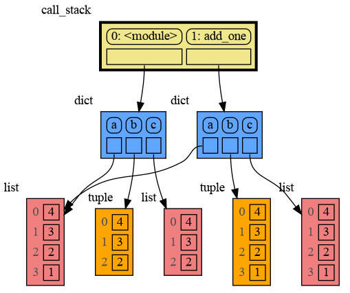
The mg.stack() function retrieves the entire call stack, including the local variables for each function on the stack. This enables us to understand function calls, variable scope, and the complete program state through call stack visualization. By examining the graph, we can see whether local variables from different function calls share data. For instance, consider the function add_one() which adds the value 1 to each of its parameters a, b, and c.

import memory_graph as mg

def add_one(a, b, c):
    a += [1]
    b += (1,)
    c += [1]
    mg.show(mg.stack())

a = [4, 3, 2]
b = (4, 3, 2)
c = [4, 3, 2]
add_one(a, b, c.copy())

print(f"a:{a} b:{b} c:{c}")

Or see it in the Memory Grah Web Debugger.

In the printed output we see that only a is changed as a result of the function call:

a:[4, 3, 2, 1] b:(4, 3, 2) c:[4, 3, 2]

This is because b is of immutable type 'tuple' so its value gets copied automatically when it is changed. And because the function is called with a copy of c, its original value is not changed by the function. The value of variable a is the only value of mutable type that is shared between the root stack frame '0: <module>' and the '1: add_one' stack frame of the function call so only that variable is affected as a result of calling the function. The other changes remain confined to the local variables of the add_one() function.

Function Call That Changes 'int' Value

Even though int is an immutable type, so an int value can not be changed by directly passing it to a function, we can still change it by wrapping it in a mutable container.

import memory_graph as mg

def add_one(a, b):
    a += 1     # change remains confined to 'a' in the add_one function
    b[0] += 1  # change also affects 'b' outside of the add_one function
    mg.show(mg.stack())

a = 10
b = [10]  # wrap in a value of mutable type list
add_one(a, b)

print(f"a:{a} b:{b[0]}")

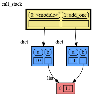
a:10 b:11

Or see it in the Memory Grah Web Debugger

The effect of calling add_one() is that b[0] increases by 1, while a is unaffected.

Data Model Exercises

Now is a good time to practice with Python Data Model concepts. Here are some exercises on references, mutability, copies, and function calls.

Block

It is often helpful to temporarily block program execution to inspect the graph. For this we can use the mg.block() function:

mg.block(fun, arg1, arg2, ...) 

This function:

• first executes fun(arg1, arg2, ...)
• then prints the current source location in the program
• then blocks execution until the <Enter> key is pressed
• finally returns the return value of the fun() call

Recursion

The call stack is also helpful to visualize how recursion works. Here we use mg.block() to show each step of how recursively factorial(4) is computed:

import memory_graph as mg

def factorial(n):
    mg.block(mg.show, mg.stack())
    if n==0:
        return 1
    result = n * factorial(n-1)
    mg.block(mg.show, mg.stack())
    return result

print( factorial(4) )

and the result is: 1 x 2 x 3 x 4 = 24

Or see it in the Memory Grah Web Debugger.

Binary Conversion

A more interesting recursive example is function binary() that converts a integer from decimal to binary representation.

import memory_graph as mg
mg.config.type_to_horizontal[list] = True  # horizontal lists

def binary(value: int) -> list[int]:
    mg.block(mg.show(), mg.stack())
    if value == 0:
        return []
    quotient, remainder = divmod(value, 2)
    result = binary(quotient) + [remainder]
    mg.block(mg.show(), mg.stack())
    return result

print( binary(100) )

[1, 1, 0, 0, 1, 0, 0]

Or see it in the Memory Grah Web Debugger.

Power Set

A more complex recursive example is function power_set() where lists are shared by different function calls. A power set is the set of all subsets of a collection of values.

import memory_graph as mg

def get_subsets(subsets, data, i, subset):
    mg.block(mg.show, mg.stack())
    if i == len(data):
        subsets.append(subset.copy())
        return
    subset.append(data[i])
    get_subsets(subsets, data, i+1, subset)  #    do include data[i]
    subset.pop()
    get_subsets(subsets, data, i+1, subset)  # don't include data[i]
    mg.block(mg.show, mg.stack())

def power_set(data):
    subsets = []
    get_subsets(subsets, data, 0, [])
    return subsets

print( power_set(['a', 'b', 'c']) )

[['a', 'b', 'c'], ['a', 'b'], ['a', 'c'], ['a'], ['b', 'c'], ['b'], ['c'], []]

Or see it in the Memory Grah Web Debugger.

Invocation Tree

The memory_graph package visualizes data at the currect time, but to better understand recursion it can also be helpful to visualize different function calls over time. This is what the invocation_tree package does.

See the power_set example in the Invocation Tree Web Debugger.

Debugging

For the best debugging experience with memory_graph set for example expression:

mg.render(locals(), "my_graph.pdf")

as a watch in a debugger tool such as the integrated debugger in Visual Studio Code. Then open the "my_graph.pdf" output file to continuously see all the local variables while debugging. This avoids having to add any memory_graph show() or render() calls to your code.

Call Stack in Watch Context

The mg.stack() doesn't work well in watch context in most debuggers because debuggers introduce additional stack frames that cause problems. Use these alternative functions for various debuggers to filter out these problematic stack frames:

debugger	function to get the call stack in 'watch' context
pdb, pudb	mg.stack_pdb()
Visual Studio Code	mg.stack_vscode()
Cursor AI	mg.stack_cursor()
PyCharm	mg.stack_pycharm()
Wing	mg.stack_wing()

See the Quick Intro (3:49) video for the setup.

Other Debuggers

For other debuggers, invoke this function within the watch context. Then, in the "call_stack.txt" file, identify the slice of functions you wish to include as stack frames in the call stack.

mg.save_call_stack("call_stack.txt")

Then to get the call stack use:

mg.stack_slice(begin_functions : list[(str,int)] = [],
               end_functions : list[str] = ["<module>"],
               stack_index: int = 0)

with these parameters that determine the begin and end index of the slice of stack frames in the call stack:

• begin_functions: list of (function-name, offset), begins at the index of the first 'function-name' that is found in the call stack with additional 'offset', otherwise begins at index 0
• end_functions: list of function-names, ends at the index of the first 'function-name' that is found in the call stack after begin index (inclusive), otherwise ends at the last index
• stack_index: number of frames removed at the beginning

Debugging without Debugger Tool

To simplify debugging without a debugger tool, we offer these alias functions that you can insert into your code at the point where you want to visualize a graph:

alias	purpose	function call
mg.sl()	show local variables	mg.show(locals())
mg.ss()	show the call stack	mg.show(mg.stack())
mg.bsl()	block after showing local variables	mg.block(mg.show, locals())
mg.bss()	block after showing the call stack	mg.block(mg.show, mg.stack())
mg.rl()	render local variables	mg.render(locals())
mg.rs()	render the call stack	mg.render(mg.stack())
mg.brl()	block after rendering local variables	mg.block(mg.render, locals())
mg.brs()	block after rendering the call stack	mg.block(mg.render, mg.stack())
mg.l()	same as mg.bsl()
mg.s()	same as mg.bss()

For example, executing this program:

from memory_graph as mg

squares = []
squares_collector = []
for i in range(1, 6):
    squares.append(i**2)
    squares_collector.append(squares.copy())
    mg.l() # block after showing local variables

and pressing <Enter> a number of times, results in:

Data Structure Examples

Package memory_graph can visualize the structure of your data to easily understand and debug data structures, some examples:

Circular Doubly Linked List

import memory_graph as mg
import random
random.seed(0)  # use same random numbers each run

class Linked_List:
    """ Circular doubly linked list """

    def __init__(self, value=None, 
                 prev=None, next=None):
        self.prev = prev if prev else self
        self.value = value
        self.next = next if next else self

    def add_back(self, value):
        if self.value == None:
            self.value = value 
        else:
            new_node = Linked_List(value,
                                   prev=self.prev,
                                   next=self)
            self.prev.next = new_node
            self.prev = new_node

linked_list = Linked_List()
n = 100
for i in range(n):
    value = random.randrange(n)
    linked_list.add_back(value)
    mg.block(mg.show, locals())  # <--- draw locals

Linked List in Cursor AI

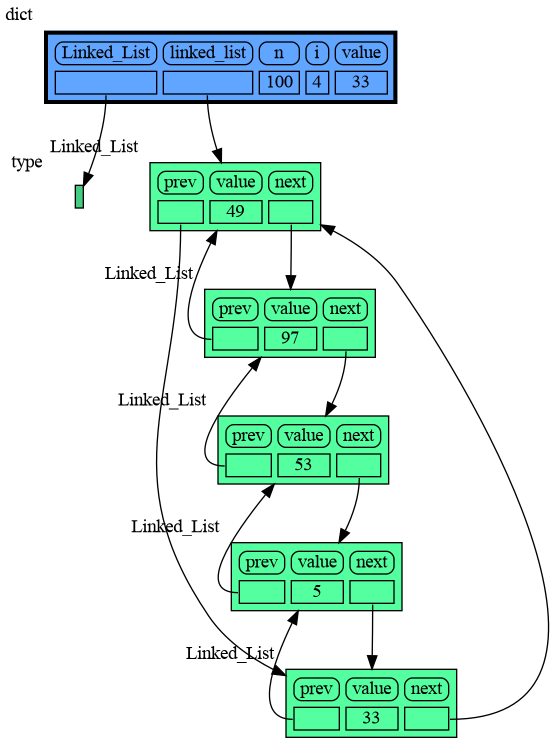
Here we show values being added to a Linked List in Cursor AI. When adding the last value '5' we "Step Into" the code to show more of the details.

Or see it in the Memory Grah Web Debugger.

Binary Tree

import memory_graph as mg
import random
random.seed(0) # use same random numbers each run

class BinTree:

    def __init__(self, value=None, smaller=None, larger=None):
        self.smaller = smaller
        self.value = value
        self.larger = larger

    def add(self, value):
        if self.value is None:
            self.value = value
        elif value < self.value:
            if self.smaller is None:
                self.smaller = BinTree(value)
            else:
                self.smaller.add(value)
        else:
            if self.larger is None:
                self.larger = BinTree(value)
            else:
                self.larger.add(value)
        mg.block(mg.show, mg.stack())  # <--- draw stack

tree = BinTree()
n = 100
for i in range(n):
    value = random.randrange(n)
    tree.add(value)

Binary Tree in Visual Studio Code

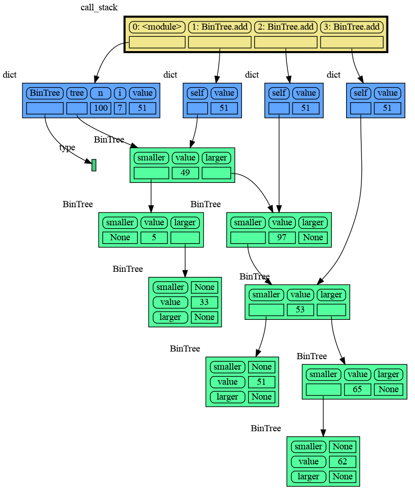
Here we show values being inserted in a Binary Tree in Visual Studio Code. When inserting the last value '29' we "Step Into" the code to show the recursive implementation.

See it in the Memory Grah Web Debugger or see the more advanced Multiway Tree with more than two children per node, making the tree less deep and more efficient.

Hash Set

import memory_graph as mg
import random
random.seed(0)  # use same random numbers each run

class HashSet:

    def __init__(self, capacity=15):
        self.buckets = [None] * capacity

    def add(self, value):
        index = hash(value) % len(self.buckets)
        if self.buckets[index] is None:
            self.buckets[index] = []
        bucket = self.buckets[index]
        bucket.append(value)
        mg.block(mg.show, locals())  # <--- draw locals

    def contains(self, value):
        index = hash(value) % len(self.buckets)
        if self.buckets[index] is None:
            return False
        return value in self.buckets[index]

    def remove(self, value):
        index = hash(value) % len(self.buckets)
        if self.buckets[index] is not None:
            self.buckets[index].remove(value)
        
hash_set = HashSet()
n = 100
for i in range(n):
    new_value = random.randrange(n)
    hash_set.add(new_value)

Hash Set in PyCharm

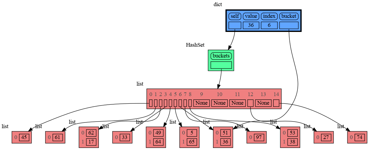
Here we show values being inserted in a HashSet in PyCharm. When inserting the last value '44' we "Step Into" the code to show more of the details.

Or see it in the Memory Grah Web Debugger.

Sorting Algorithms

Visualization of different sorting algorithms in Memory Graph Web Debugger.

• selection sort
• insertion sort
• bubble sort
• cocktail shaker sort

Bitwise Operators

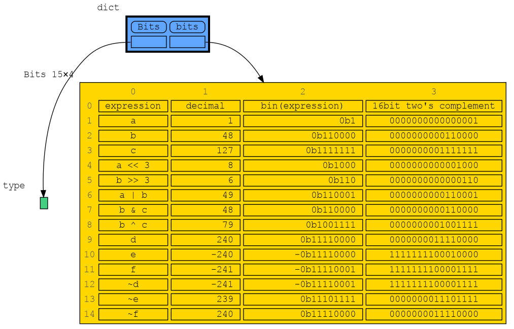
In this configuration example we show the decimal, binary and two's complement representation representation of int values of dictionary subclass Bits to show the result of bitwise operators. The ~ (inverse) operator can be a bit confusing if not shown with two's complement representation.

• bitwise operators

Sliding Puzzle Solver

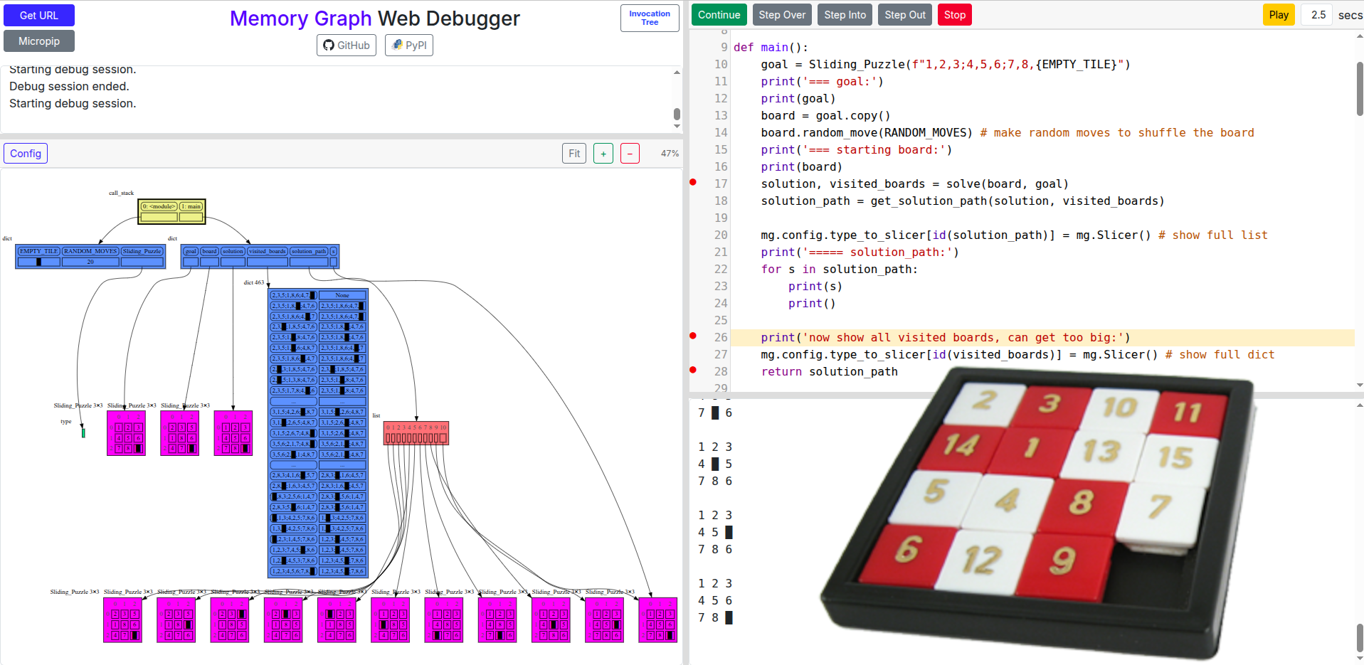
A sliding puzzle solver as a challenging example showing how memory_graph deals with large amounts of data. Click "Continue" to step through the breadth-first search generations until a solution path is found:

• sliding puzzle solver

Configuration

Different aspects of memory_graph can be configured. The default configuration can be reset by calling 'mg.config_default.reset()'. The Memory Graph Web Debugger gives examples of the most important configurations.

• mg.config.reopen_viewer : bool

  • If True the viewer is reopened each time show() is called, this might change window focus, default True.

• mg.config.render_filename : str

  • The default filename to render to, default 'memory_graph.pdf'.

• mg.config.type_labels : bool

  • If True the type of each node is shown as label, default True.

• mg.config.block_prints_location : bool

  • If True the source location is printed in block(), default True.

• mg.config.press_enter_message : str

  • Message to ask user to press <Enter> in block(), set to None to disable.

• mg.config.max_string_length : int

  • The maximum length of strings shown in the graph. Longer strings will be truncated.

• mg.config.embedded_types : set[type]

  • Holds all types for which no separate node is drawn but that are embedded in their parent Node.

• mg.config.embedded_key_types : set[type]

  • Holds all types that are embedded as key in a Node_Key_Value node, even when not in 'embedded_types'.

• mg.config.embedding_types : set[type]

  • Holds all dictionary types that embed their key-value tuple children.

• mg.config.no_index_types : set[type]

  • Holds all types like 'set' and 'frozenset' that should not have indices as Node_Linear.

• mg.config.type_to_node : dict[type, fun(data) -> Node]

  • Determines how a data type is converted to a Node subclass for visualization in the graph.

• mg.config.type_to_color : dict[type, color]

  • Maps a type to the graphviz color it gets in the graph.

• mg.config.type_to_horizontal : dict[type, bool]

  • Maps a type to its orientation for Node_Linear and Node_Key_Value. Use 'True' for horizontal and 'False' for vertical. If not specified these nodes vertical unless they have references to children.

• mg.config.type_to_slicer : dict[type, int]

  • Maps a type to a Slicer. A slicer determines how many elements of a data type are shown in the graph to prevent the graph from getting too big. 'Slicer()' does no slicing, 'Slicer(1,2,3)' shows just 1 element at the beginning, 2 in the middle, and 3 at the end.

• mg.config.max_graph_depth : int

  • The maxium depth of the graph with default value 1000.

• mg.config.graph_cut_symbol : str

  • The symbol indicating where the graph is cut short with default ✂.

• mg.config.type_to_depth : dict[type, int]

  • Maps a type to graph depth to limit the graph size.

• mg.config.max_missing_edges : int

  • Maximum number of missing edges that are shown with default value 2. Dashed references are used to indicate that there are more references to a node than are shown.

• mg.config.fontname : str

  • The font used in the graph, default 'Times-Roman' (widely available on the web).

• mg.config.fontsize : str

  • The font size used in the graph, default '14'.

Simplified Graph

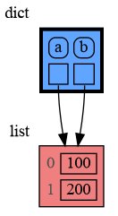
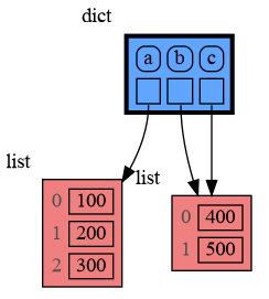
Memory_graph simplifies the visualization (and the viewer's mental model) by not showing separate nodes for immutable types like bool, int, float, complex, and str by default. This simplification can sometimes be slightly misleading. As in the example below, after a shallow copy, lists a and b technically share their int values, but the graph makes it appear as though a and b each have their own copies. However, since int is immutable, this simplification will never lead to unexpected changes (changing a won’t affect b) so will never result in bugs.

The simplification strikes a balance: it is slightly misleading but keeps the graph clean and easy to understand and focuses on the mutable types where unexpected changes can occur. This is why it is the default behavior. If you do want to show separate nodes for int values, such as for educational purposes, you can simply remove int from the mg.config.embedded_types set:

import memory_graph as mg

a = [100, 200, 300]
b = a.copy()
mg.render(locals(), 'embedded1.png')

mg.config.embedded_types.remove(int)  # now show separate nodes for int values

mg.render(locals(), 'embedded2.png')

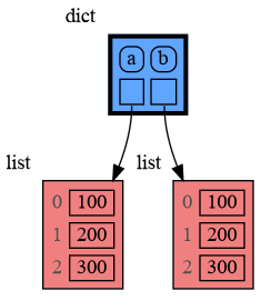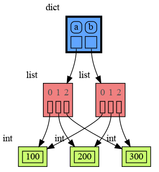embedded1.png — simplified	embedded2.png — technically correct

Additionally, the simplification hides away the reuse of small int values [-5, 256] in the current CPython implementation, an optimization that might otherwise confuse beginner Python programmers. For instance, after executing a[1]+=1; b[1]+=1 the 201 value is, maybe surprisingly, still shared between a and b, whereas executing a[2]+=1; b[2]+=1 does not result in sharing the 301 value. Similarly CPython uses String Interning to reuse small strings.

Introspection

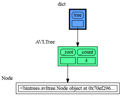
Sometimes the introspection fails or is not as desired. For example the bintrees.avltree.Node object doesn't show any attributes in the graph below.

import memory_graph as mg
import bintrees

# Create an AVL tree
tree = bintrees.AVLTree()
tree.insert(10, "ten")
tree.insert(5, "five")
tree.insert(20, "twenty")
tree.insert(15, "fifteen")

mg.show(locals())

All attributes using dir()

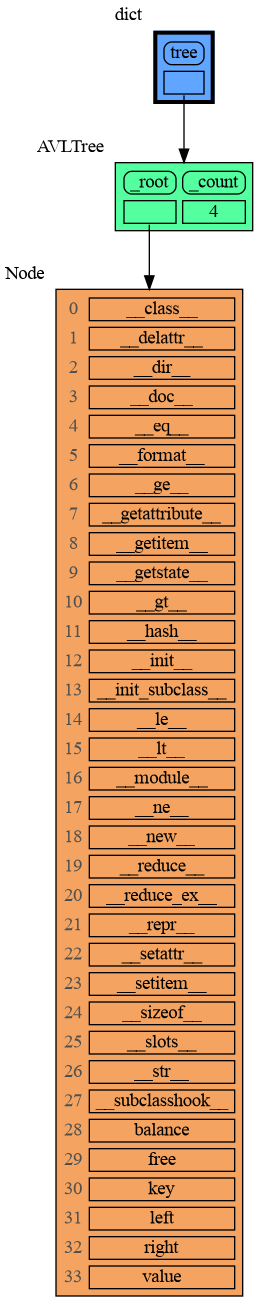
A useful start is to give it some color, show the list of all its attributes using dir(), and setting an empty Slicer to see the attribute list in full.

import memory_graph as mg
import bintrees

# Create an AVL tree
tree = bintrees.AVLTree()
tree.insert(10, "ten")
tree.insert(5, "five")
tree.insert(20, "twenty")
tree.insert(15, "fifteen")

mg.config.type_to_color[bintrees.avltree.Node] = "sandybrown"
mg.config.type_to_node[bintrees.avltree.Node] = lambda data: mg.Node_Linear(data,
                                                dir(data))
mg.config.type_to_slicer[bintrees.avltree.Node] = mg.Slicer()

mg.show(locals())

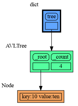
Next figure out what the attributes are you want to graph and choose a Node type, there are four options:

1) Node_Leaf

Node_Leaf is a node with no children and shows just a single value.

import memory_graph as mg
import bintrees

# Create an AVL tree
tree = bintrees.AVLTree()
tree.insert(10, "ten")
tree.insert(5, "five")
tree.insert(20, "twenty")
tree.insert(15, "fifteen")

mg.config.type_to_color[bintrees.avltree.Node] = "sandybrown"
mg.config.type_to_node[bintrees.avltree.Node] = lambda data: mg.Node_Leaf(data,
                                                f"key:{data.key} value:{data.value}")

mg.show(locals())

2) Node_Linear

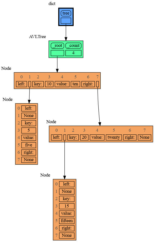
Node_Linear shows multiple values in a line like a list.

import memory_graph as mg
import bintrees

# Create an AVL tree
tree = bintrees.AVLTree()
tree.insert(10, "ten")
tree.insert(5, "five")
tree.insert(20, "twenty")
tree.insert(15, "fifteen")

mg.config.type_to_color[bintrees.avltree.Node] = "sandybrown"
mg.config.type_to_node[bintrees.avltree.Node] = lambda data: mg.Node_Linear(data,
                                                ['left:', data.left,
                                                 'key:', data.key,
                                                 'value:', data.value,
                                                 'right:', data.right] )

mg.show(locals())

3) Node_Key_Value

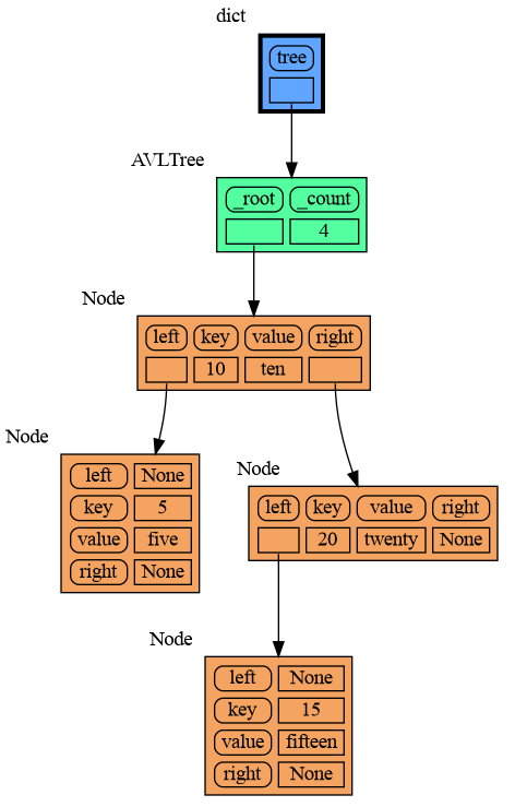
Node_Key_Value shows key-value pairs like a dictionary. Note the required items() call at the end.

import memory_graph as mg
import bintrees

# Create an AVL tree
tree = bintrees.AVLTree()
tree.insert(10, "ten")
tree.insert(5, "five")
tree.insert(20, "twenty")
tree.insert(15, "fifteen")

mg.config.type_to_color[bintrees.avltree.Node] = "sandybrown"
mg.config.type_to_node[bintrees.avltree.Node] = lambda data: mg.Node_Key_Value(data,
                                                {'left': data.left,
                                                 'key': data.key,
                                                 'value': data.value,
                                                 'right': data.right}.items() )

mg.show(locals())

4) Node_Table

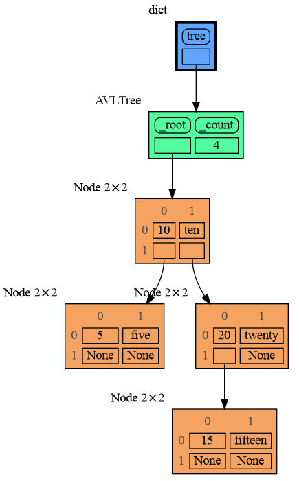
Node_Table shows all the values as a table.

import memory_graph as mg
import bintrees

# Create an AVL tree
tree = bintrees.AVLTree()
tree.insert(10, "ten")
tree.insert(5, "five")
tree.insert(20, "twenty")
tree.insert(15, "fifteen")

mg.config.type_to_color[bintrees.avltree.Node] = "sandybrown"
mg.config.type_to_node[bintrees.avltree.Node] = lambda data: mg.Node_Table(data,
                                                [[data.key, data.value],
                                                 [data.left, data.right]] )

mg.show(locals())

Binary Search

For binary search we can use a List_View class to represent a particular sublist without making a list copy.

import memory_graph as mg
import random
random.seed(2)  # same random numbers each run

class List_View:

    def __init__(self, lst, begin, end):
        self.lst = lst
        self.begin = begin
        self.end = end

    def __getitem__(self, index):
        return self.lst[index]

    def get_mid(self):
        return (self.begin + self.end) // 2

def bin_search(view, value):
    mid = view.get_mid()
    if view.begin == mid:
        mg.show(mg.stack())  # <--- show stack
        return view.begin
    if value < view[mid]:
        return bin_search(List_View(view.lst, view.begin, mid), value)
    else:
        return bin_search(List_View(view.lst, mid, view.end), value)

# create sorted list
n = 15
data = [random.randrange(1000) for _ in range(n)]
data.sort()

# search 'value'
value = data[random.randrange(n)]
index = bin_search(List_View(data, 0, len(data)), value)
print('index:', index, 'data[index]:', data[index])

Arguably the visualization is then more clear when we show a List_View object as an actual sublist using a Node_linear node:

mg.config.type_to_node[List_View] = (lambda l: mg.Node_Linear(l,
    [v if l.begin <= i < l.end else '' for i, v in enumerate(l.lst)]
    if hasattr(l, 'end') else [])
)

Graph Depth

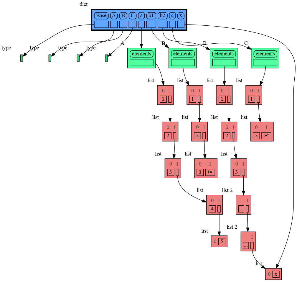
To limit the size of the graph the maximum depth of the graph is set by mg.config.max_graph_depth. Additionally for each type a depth can be set to further limit the graph, as is done for type B in the example below. Scissors indicate where the graph is cut short. Alternatively the id() of a data elements can be used to limit the graph for that specific element, as is done for the value referenced by variable c.

The value of variable x is shown as it is at depth 1 from the root of the graph, but as it can also be reached via b2, that path need to be shown as well to avoid confusion, so this overwrites the depth limit set for type B.

import memory_graph as mg

class Base:

    def __init__(self, n):
        self.elements = [1]
        iter = self.elements
        for i in range(2,n):
            iter.append([i])
            iter = iter[-1]

    def get_last(self):
        iter = self.elements
        while len(iter)>1:
            iter = iter[-1]
        return iter

class A(Base):

    def __init__(self, n):
        super().__init__(n)

class B(Base):

    def __init__(self, n):
        super().__init__(n)

class C(Base):

    def __init__(self, n):
        super().__init__(n)

a = A(6)
b1 = B(6)
b2 = B(6)
c = C(6)

x = ['x']
b2.get_last().append(x)

mg.config.type_to_depth[B] = 3
mg.config.type_to_depth[id(c)] = 2
mg.show(locals())

Hidden Edges

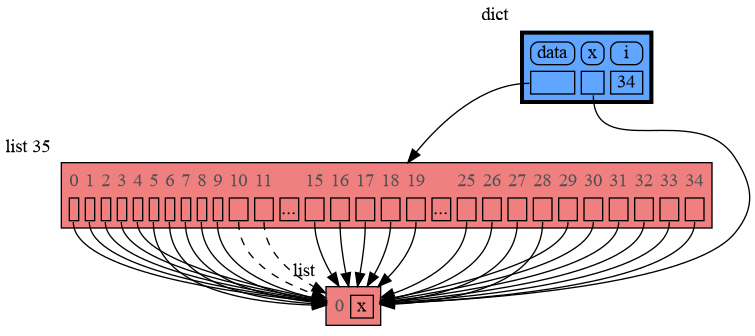
As the value of x is shown in the graph, we would want to show all the references to it, but the default list Slicer hides references by slicing the list to keep the graph small. The max_missing_edges variable then determines how many additional hidden references to x we show. If there are more references then we show, then theses hidden references are shown with dashed lines to indicate some references are left out.

import memory_graph as mg

data = []
x = ['x']
for i in range(20):
    data.append(x)

mg.show(locals())

Extensions

Different extensions are available for types from other Python packages.

Numpy

Numpy types array and matrix and ndarray can be graphed with "memory_graph.extension_numpy":

import memory_graph as mg
import numpy as np
import memory_graph.extension_numpy
np.random.seed(0) # use same random numbers each run

matrix = np.matrix([[i*5+j for j in range(4)] for i in range(5)])
ndarray_1d = np.array([1.1, 2, 3, 4, 5])
ndarray_2d = np.random.rand(3,2)
ndarray_3d = np.random.rand(2,2,2)

mg.show(locals())

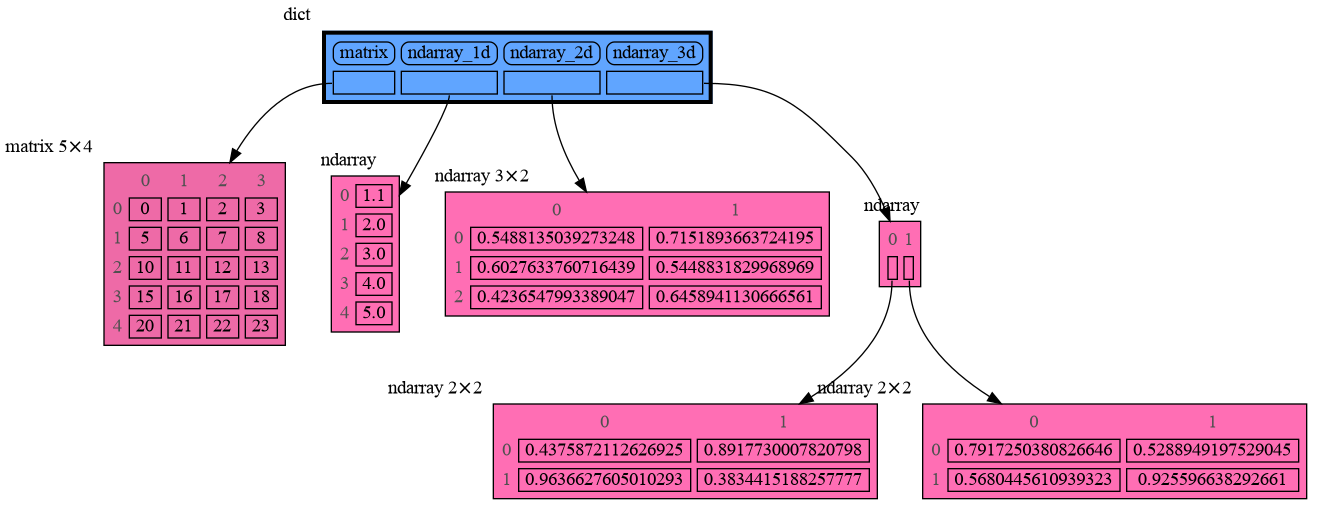
Or see it in the Memory Grah Web Debugger.

Pandas

Pandas types Series and DataFrame can be graphed with "memory_graph.extension_pandas":

import memory_graph as mg
import pandas as pd
import memory_graph.extension_pandas

series = pd.Series( [i for i in range(20)] )
dataframe1 = pd.DataFrame({  "calories": [420, 380, 390],
                             "duration": [50, 40, 45] })
dataframe2 = pd.DataFrame({  'Name'   : [ 'Tom', 'Anna', 'Steve', 'Lisa'],
                             'Age'    : [    28,     34,      29,     42],
                             'Length' : [  1.70,   1.66,    1.82,   1.73] },
                            index=['one', 'two', 'three', 'four']) # with row names
mg.show(locals())

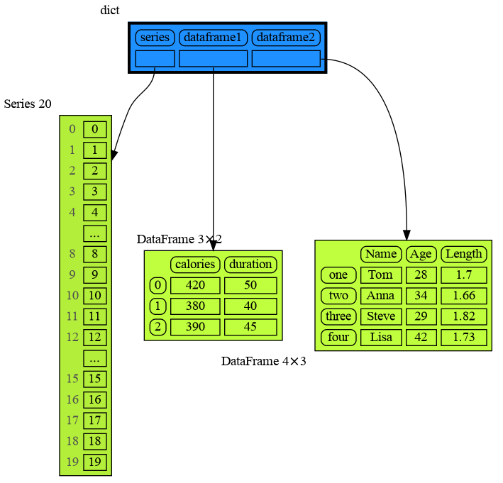
Or see it in the Memory Grah Web Debugger.

PyTorch

Torch type tensor can be graphed with "memory_graph.extension_torch":

import memory_graph as mg
import torch
import memory_graph.extension_torch
torch.manual_seed(0) # same random numbers each run

tensor_1d = torch.rand(3)
tensor_2d = torch.rand(3, 2)
tensor_3d = torch.rand(2, 2, 2)

mg.show(locals())

Memory Graph Web Debugger

The Memory Graph Web Debugger lets us use memory_graph without any installation.

Jupyter Notebook

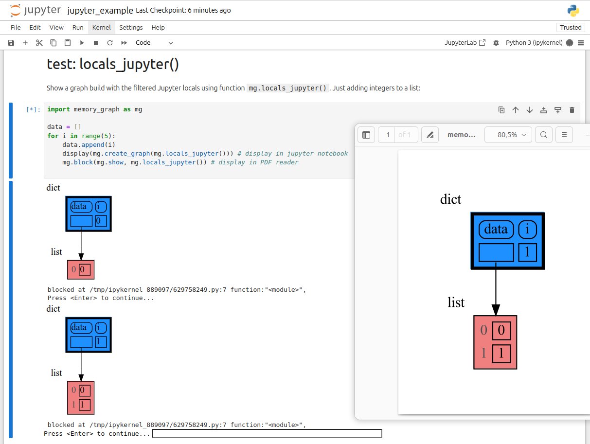
In Jupyter Notebook locals() has additional variables that cause problems in the graph, use mg.locals_jupyter() to get the local variables with these problematic variables filtered out. Use mg.stack_jupyter() to get the whole call stack with these variables filtered out.

We can use mg.show() and mg.render() in a Jupyter Notebook, but alternatively we can also use mg.create_graph() to create a graph and the display() function to render it inline with for example:

display( mg.create_graph(mg.locals_jupyter()) ) # display the local variables inline
mg.block(display, mg.create_graph(mg.locals_jupyter()) ) # the same but blocked

See for example jupyter_example.ipynb.

ipython

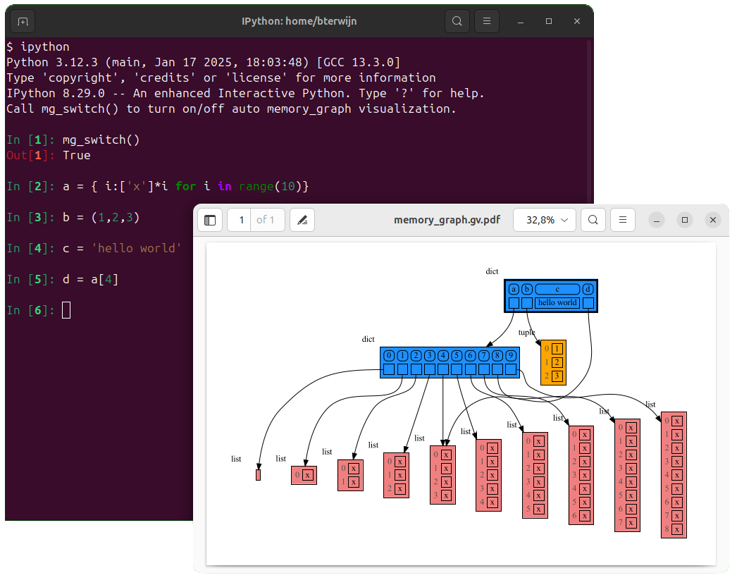
In ipython locals() has additional variables that cause problems in the graph, use mg.locals_ipython() to get the local variables with these problematic variables filtered out. Use mg.stack_ipython() to get the whole call stack with these variables filtered out.

Additionally install file auto_memory_graph.py in the ipython startup directory:

• Linux/Mac: ~/.ipython/profile_default/startup/
• Windows: %USERPROFILE%\.ipython\profile_default\startup\

Then after starting 'ipython' call function mg_switch() to turn on/off the automatic visualization of local variables after each command.

Google Colab

In Google Colab locals() has additional variables that cause problems in the graph, use mg.locals_colab() to get the local variables with these problematic variables filtered out. Use mg.stack_colab() to get the whole call stack with these variables filtered out.

See for example colab_example.ipynb.

Marimo

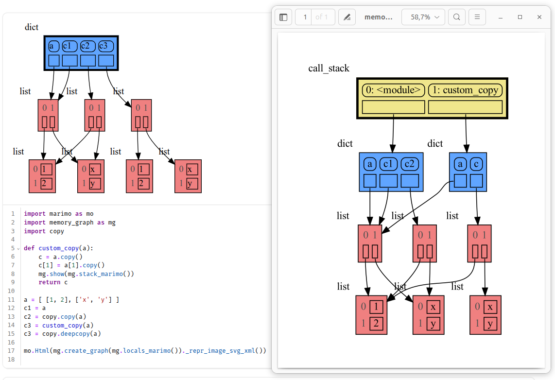
In Marimo locals() has additional variables that cause problems in the graph, use mg.locals_marimo() to get the local variables with these problematic variables filtered out. Use mg.stack_marimo() to get the whole call stack with these variables filtered out. Memory_graph only works when running Marimo locally, not in the playground.

See for example marimo_example.py.

Animated GIF

To make an animated GIF use for example mg.show or mg.render like this:

• mg.show(locals(), 'animated.png', numbered=True)
• mg.render(locals(), 'animated.png', numbered=True)

in your source or better as a watch in a debugger so that stepping through the code generates images:

    animated0.png, animated1.png, animated2.png, ...

Then use these images to make an animated GIF, for example using this Bash script create_gif.sh:

$ bash create_gif.sh animated

Troubleshooting

• Adobe Acrobat Reader doesn't refresh a PDF file when it changes on disk and blocks updates which results in an Could not open 'memory_graph.pdf' for writing : Permission denied error. One solution is to install a PDF reader that does refresh (SumatraPDF, Okular, ...) and set it as your default PDF reader. Another solution is to render() the graph to a different output format.

• When graph edges overlap it can be hard to distinguish them. Using an interactive graphviz viewer, such as xdot, on a '*.gv' DOT output file will help.

Other Packages

The memory_graph package visualizes your data. If instead you want to visualize function calls, check out the invocation_tree package.