


Model-Structured Neural Networks for modeling, control and estimation of physical systems
Modeling, control, and estimation of physical systems are central to many engineering disciplines. While data-driven methods like neural networks offer powerful tools, they often struggle to incorporate prior domain knowledge, limiting their interpretability, generalizability, and safety.
To bridge this gap, we present nnodely (where "nn" can be read as "m," forming Modely) — a framework that facilitates the creation and deployment of Model-Structured Neural Networks (MS-NNs).
MS-NNs combine the learning capabilities of neural networks with structural priors grounded in physics, control and estimation theory, enabling:
- Reduced training data requirements
- Generalization to unseen scenarios
- Real-time deployment in real-world applications
Why use nnodely?
The framework's goal is to allow fast prototyping of MS-NNs for modeling, control and estimation of physical systems, by embedding prior domain knowledge into the neural networks' architecture.
Core Objectives
- Model, control, or estimate physical systems with unknown internal dynamics or parameters.
- Accelerate the development of MS-NNs, which are often hard to implement in general-purpose deep learning frameworks.
- Support researchers, engineers and domain experts to integrate data-driven models into their workflow — without discarding established knowledge.
- Serve as a repository of reusable components and best practices for MS-NN design across diverse applications.
Workflow Overview
nnodely guides users through six structured phases to define, train, and deploy MS-NNs effectively:
- Neural Model Definition: Build the MS-NN architecture using intuitive and modular design functions.
- Dataset Creation: Simplify loading and preprocessing of training, validation, and test data.
- Neural Model Composition: Assemble complex models by combining multiple neural components (e.g., models, controllers, estimators) in a unified training framework.
- Neural Model Training: Train the MS-NN's parameters with user-defined loss functions.
- Neural Model Validation: Assess the performance and reliability of the trained model.
- Model Export: Deploy MS-NNs using standard formats. nnodely supports export to native PyTorch (nnodely-independent) and ONNX for broader compatibility.
Table of Contents
Getting Started
You can install the nnodely framework from PyPI via:
pip install nnodely
Applications and use cases
Some examples of application of nnodely in different fields are collected in the following open-source repository: nnodely-applications
How to contribute
Download the source code and install the dependencies using the following commands:
git clone git@github.com:tonegas/nnodely.git
pip install -r requirements.txt
To contribute to the nnodely framework, you can:
- Open a pull request, if you have a new feature or bug fix.
- Open an issue, if you have a question or suggestion.
We are very happy to collaborate with you!
(back to top)
Basic Example
This example shows how to use nnodely to create a model-structured neural network (MS-NN) for a simple mass-spring-damper mechanical system.
Build the neural model
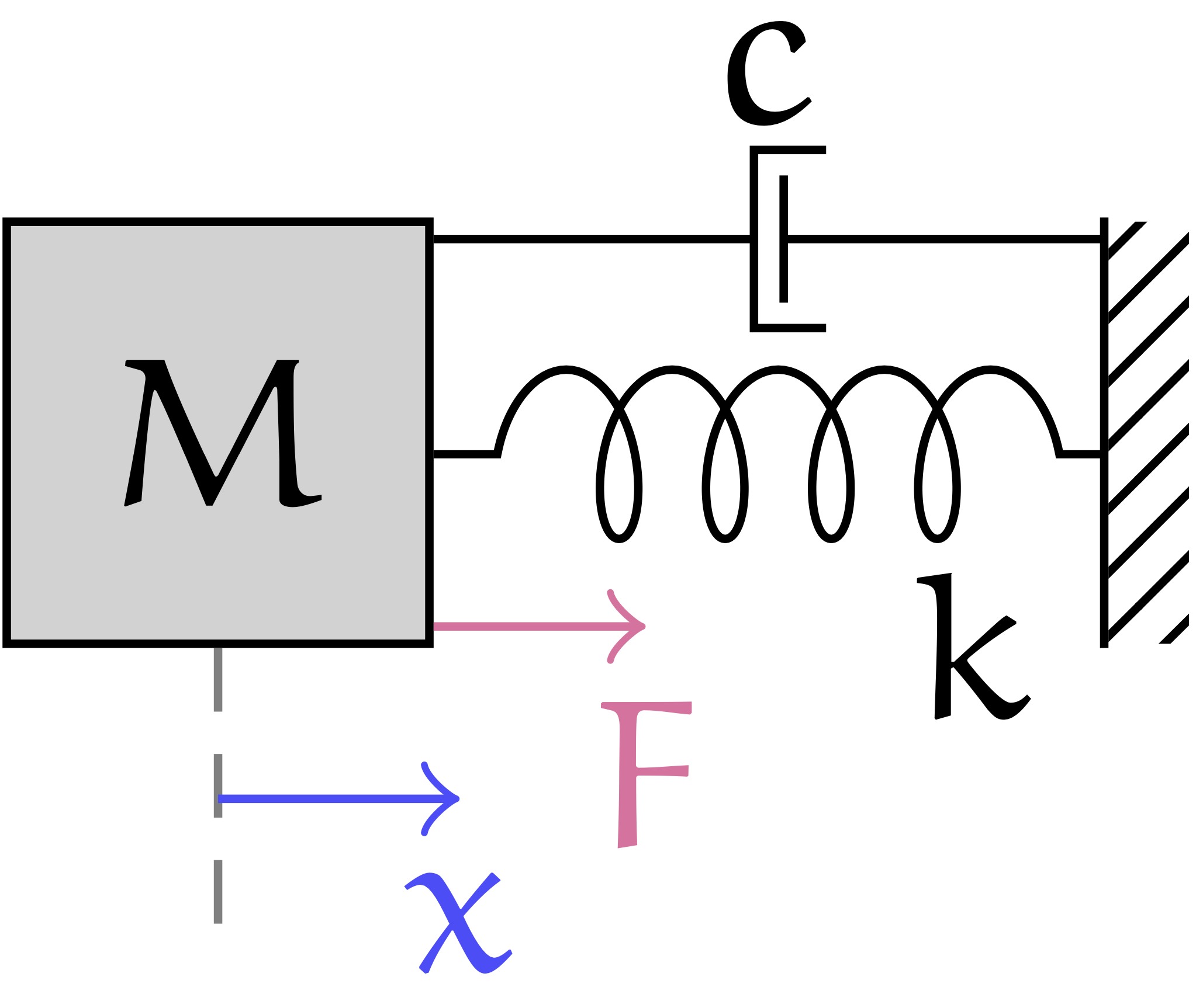
The system to be modeled is defined by the following equation:
M \ddot x = - k x - c \dot x + F
Suppose we want to estimate the value of the future position of the mass, given the initial position and the external force.
The MS-NN model is defined by a list of inputs and outputs, and by a list of relationships that link the inputs to the outputs.
In nnodely, we can build an estimator in this form:
x = Input('x')
F = Input('F')
x_z_est = Output('x_z_est', Fir(x.tw(1)) + Fir(F.last()))
Input variables can be created using the Input function.
In our system, we have two inputs: the position of the mass, x, and the external force exerted on the mass, F.
The Output function is used to define a model's output.
The Output function has two inputs: the first is the name (string) of the output, and the second is the structure of the estimator.
Let's explain some of the functions used:
- The
tw(...) function is used to extract a time window from a signal.
In particular, we extract a time window $T_w$ of 1 second.
- The
last() function that is used to get the last force sample applied to the mass, i.e., the force at the current time step.
- The
Fir(...) function to build an FIR (finite impulse response) filter with one learnable parameters on our input variable.
Hence, we are creating an estimator for the variable x at the next time step (i.e., the future position of the mass), by building an observer with the following mathematical structure:
x[1] = \sum_{k=0}^{N_x-1} x[-k]\cdot h_x[(N_x-1)-k] + F[0]\cdot h_F
where $x[1]$ is the next position of the mass, $F[0]$ is the last sample of the force, $N_x$ is the number of samples in the time window of the input variable x, $h_x$ is the vector of learnable parameters of the FIR filter on x, and $h_f$ is the single learnable parameter of the FIR filter on F.
For the input variable x, we are using a time window $T_w = 1$ second, which means that we are using the last $N_x$ samples of the variable x to estimate the next position of the mass. The value of $N_x$ is equal to $T_w/T_s$, where $T_s$ is the sampling time used to sample the input variable x.
In a particular case, our MS-NN formulation becomes equivalent to the discrete-time response (discretize with Forward-Euler) of the mass-spring-damper system. This happens when we choose the following values: $N_x = 3$, $h_x$ equal to the characteristic polynomial of the system, and $h_f = T_s^2/m$, where $T_s$ is the sampling time and $m$ is the mass of the system.
However, our formulation is more general and can take better adapt to model mismatches and noise levels in the measured variables. This improved learning potential can be achieved by using a larger number of samples $N_x$ in the time window of the input variable x.
Neuralize the model
Let's now try to train our MS-NN observer using the data we have.
We perform:
mass_spring_damper = Modely()
mass_spring_damper.addModel('x_z_est', x_z_est)
mass_spring_damper.addMinimize('next-pos', x.z(-1), x_z_est, 'mse')
mass_spring_damper.neuralizeModel(0.2)
The first line creates a nnodely object, while the second line adds one output to the model using the addModel function.
To train our model, we use the function addMinimize to add a loss function to the list of losses. This function uses the following inputs:
- The first input is the name of the error (
'next-pos' in this case).
- The second and third inputs are the variables whose difference we want to minimize.
- The fourth input is the loss function to be used, in this case the mean square error ('mse').
In the function addMinimize, we apply the z(-1) method to the variable x to get the next position of the mass, i.e., the value of x at the next time step. Indeed, the z(-1) function uses the Z-transform notation, and z(-1) is equivalent to next() operator.
The function z(...) can be used on an Input variable to get a time-shifted value.
Hence, our training objective is to minimize the mean square error between x_z, which represents the next position of the mass, and x_z_est, which represents the output of our estimator:
\frac{1}{n} \sum_{i=0}^{n} (x_{z_i} - x_{{z\_est}_i})^2
where n represents the number of samples in the dataset.
Finally, the function neuralizeModel is used to create a discrete-time MS-NN model. The input parameter of this function is the sampling time $T_s$, and is chosen based on the data we have available. In this example, we have a sampling time of $T_s = 0.2$ seconds.
Load the dataset
The training dataset is then loaded. nnodely has access to all the files that are in a source folder.
data_struct = ['time','x','dx','F']
data_folder = './tutorials/datasets/mass-spring-damper/data/'
mass_spring_damper.loadData(name='mass_spring_dataset', source=data_folder, format=data_struct, delimiter=';')
Train the neural network
Using the loaded dataset, we now train the neural model.
mass_spring_damper.trainModel()
Test the neural model
After training the model, we can test it using a new dataset. Let us create a new simple example to test the model, using the following inputs:
sample = {'F':[0.5], 'x':[0.25, 0.26, 0.27, 0.28, 0.29]}
results = mass_spring_damper(sample)
print(results)
Note that the input variable x is a list of 5 samples, as the sampling time $T_s$ is 0.2 seconds and the time window $T_w$ of the input variable x is 1 second. For the input variable F, we have only one sample, as we are using the last sample of the force applied to the mass.
The resulting output variable is structured as follows:
>> {'x_z_est':[0.4]}
where the value represents the output of our estimator (i.e., the next position of the mass).
Our model can be tested also using a bigger time window:
sample = {'F':[0.5, 0.6], 'x':[0.25, 0.26, 0.27, 0.28, 0.29, 0.30]}
results = mass_spring_damper(sample)
print(results)
where the value of x is built using a moving time window.
The resulting model output is structured as follows:
>> {'x_z_est':[0.4, 0.42]}
Note that the same output can be obtained by calling the model using the flag sampled=True, in this way:
sample = {'F':[[0.5],[0.6]], 'x':[[0.25, 0.26, 0.27, 0.28, 0.29],[0.26, 0.27, 0.28, 0.29, 0.30]]}
results = mass_spring_damper(sample,sampled=True)
print(results)
(back to top)
Structure of the Repository
nnodely Folder
This folder contains all the nnodely library files with relative references.
The Moldey main class defined in nnodely.py, it contains all the main properties of the nnodely object and it derives from five main operators:
- composer.py contains all the functions to build the networks:
addModel, neuralizeModel, addConnection, addClosedLool etc..
- loader.py contains the function for managing the dataset, the main function is
dataLoad.
- trainer.py contains the function for train the network as the
trainModel.
- exporter.py contains all the function for import and export:
saveModel, loadModel, exportONNX etc..
- validator.py contains all the function for validate the model ad the
resultsAnalysis.
All the operators derive from Networkdefined in network.py, that contains the shared support functions for all the operators.
The folder basic contatins the main classes for the low level functionalities:
- model.py containts the pytorch template model for the structured network.
- modeldef.py containts the operation for work with the json model definition.
- loss.py contatins the loss functions.
- optimizer.py contains the optimizer calss.
- relation.py contains all the main classes from which all the layers are derived.
The other folders are:
- exporter that contains the classes for the export functions.
- support for the support functions.
- visualizer that contains all the classes related to the visualization.
- And finally the layers folder.
The layers folder contains all the layers that can be used in the MSNN.
In particular, the model structured NN is defined by Inputs, Outputs and Parameters:
- input.py contains the Input class used for create an input for the network.
- ouptut.py contains the Output class used for create an output for the network.
- parameter.py contains the logic for create a generic parameters and constants.
The main basic layers without parameters are:
- activation.py this file contains all the activation functions. The activation are mainly based on the pytorch functions.
- arithmetic.py this file contains the aritmetic functions as: +, -, /, *., **.
- trigonometric.py this file contains all the trigonometric functions.
- part.py are used for selecting part of the data.
- fuzzify.py contains the operation for the fuzzification of a variable,
commonly used in the local model as activation function as in [1] with rectangular activation functions or in [3], [4] and [5] with triangular activation function activation functions.
Using fuzzification it is also possible create a channel coding as presented in [2].
The main basic layers with parameters are:
- fir.py this file contains the finite inpulse response filter function. It is a linear operation on the time dimension (second dimension).
This filter was introduced in [1].
- linear.py this file contains the linear function. Typical Linear operation
W*x+b operated on the space dimension (third dimension).
This operation is presented in [1].
- localmodel.py this file contains the logic for build a local model. This operation is presented in [1], [3], [4] and [5].
- parametricfunction.py are the user custom function. The function can use the pytorch syntax. A parametric function is presented in [3], [4], [5].
- equationlearner.py contains the logic for the equation learner. The equation learner is used for learn a relation input outpur following a list of activation functions. The first implementation is presented in [6].
- timeoperation.py contains the time operation functions. The time operation are used for extract a time window from a signal. The derivative operation can be used to implement Physics-informed neural network [7] Sobolev learning [8].
Tests Folder
This folder contains the unit tests of the library. Each file tests a specific functionality.
Examples Folder
The files in the examples folder are a collection of the functionality of the library.
Each file presents a specific functionality of the framework.
This folder is useful to understand the flexibility and capability of the framework.
(back to top)
License
This project is released under the license License: MIT.
(back to top)
References
[1]
Mauro Da Lio, Daniele Bortoluzzi, Gastone Pietro Rosati Papini. (2019).
Modelling longitudinal vehicle dynamics with neural networks.
Vehicle System Dynamics. https://doi.org/10.1080/00423114.2019.1638947 (look the [code])
[2]
Alice Plebe, Mauro Da Lio, Daniele Bortoluzzi. (2019).
On Reliable Neural Network Sensorimotor Control in Autonomous Vehicles.
IEEE Transaction on Intelligent Trasportation System. https://doi.org/10.1109/TITS.2019.2896375
[3]
Mauro Da Lio, Riccardo Donà, Gastone Pietro Rosati Papini, Francesco Biral, Henrik Svensson. (2020).
A Mental Simulation Approach for Learning Neural-Network Predictive Control (in Self-Driving Cars).
IEEE Access. https://doi.org/10.1109/ACCESS.2020.3032780 (look the [code])
[4]
Edoardo Pagot, Mattia Piccinini, Enrico Bertolazzi, Francesco Biral. (2023).
Fast Planning and Tracking of Complex Autonomous Parking Maneuvers With Optimal Control and Pseudo-Neural Networks.
IEEE Access. https://doi.org/10.1109/ACCESS.2023.3330431 (look the [code])
[5]
Mattia Piccinini, Sebastiano Taddei, Matteo Larcher, Mattia Piazza, Francesco Biral. (2023).
A Physics-Driven Artificial Agent for Online Time-Optimal Vehicle Motion Planning and Control.
IEEE Access. https://doi.org/10.1109/ACCESS.2023.3274836 (look [code basic]
and [code extended])
[6]
Hector Perez-Villeda, Justus Piater, Matteo Saveriano. (2023).
Learning and extrapolation of robotic skills using task-parameterized equation learner networks.
Robotics and Autonomous Systems. https://doi.org/10.1016/j.robot.2022.104309 (look the [code])
[7]
M. Raissi. P. Perdikaris b, G.E. Karniadakis a. (2019).
Physics-informed neural networks: A deep learning framework for solving forward and inverse problems involving nonlinear partial differential equations
Journal of Computational Physics. https://doi.org/10.1016/j.jcp.2018.10.045 (look the [example Burger's equation])
[8]
Wojciech Marian Czarnecki, Simon Osindero, Max Jaderberg, Grzegorz Świrszcz, Razvan Pascanu. (2017).
Sobolev Training for Neural Networks.
arXiv. https://doi.org/10.48550/arXiv.1706.04859 (look the [code])
[9]
Mattia Piccinini, Matteo Zumerle, Johannes Betz, Gastone Pietro Rosati Papini. (2025).
A Road Friction-Aware Anti-Lock Braking System Based on Model-Structured Neural Networks.
IEEE Open Journal of Intelligent Transportation Systems. https://doi.org/10.1109/OJITS.2025.3563347 (look at the [code])
[10]
Mauro Da Lio, Mattia Piccinini, Francesco Biral. (2023).
Robust and Sample-Efficient Estimation of Vehicle Lateral Velocity Using Neural Networks With Explainable Structure Informed by Kinematic Principles.
IEEE Transactions on Intelligent Transportation Systems. https://doi.org/10.1109/TITS.2023.3303776
(back to top)