scgraph

scgraph

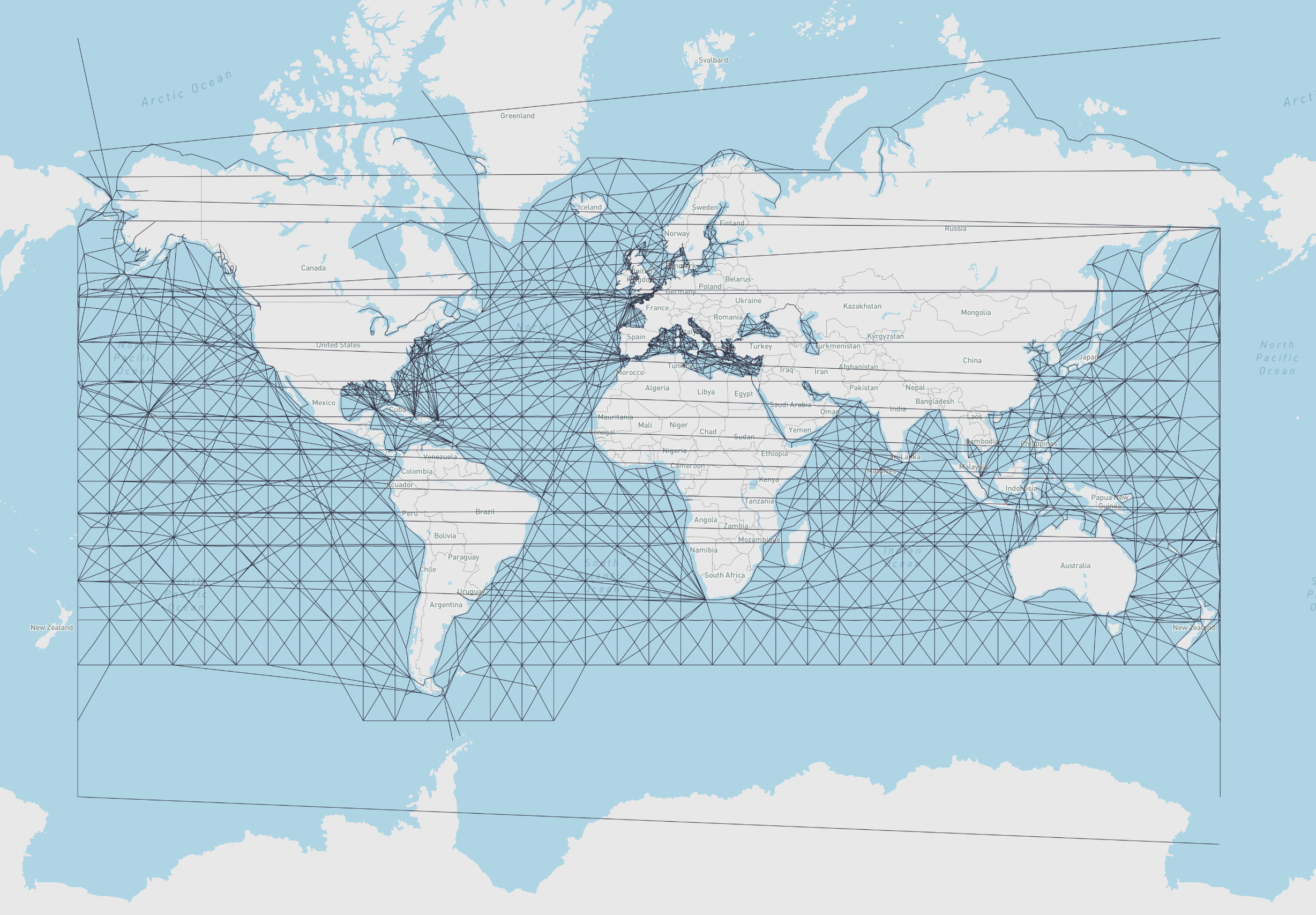
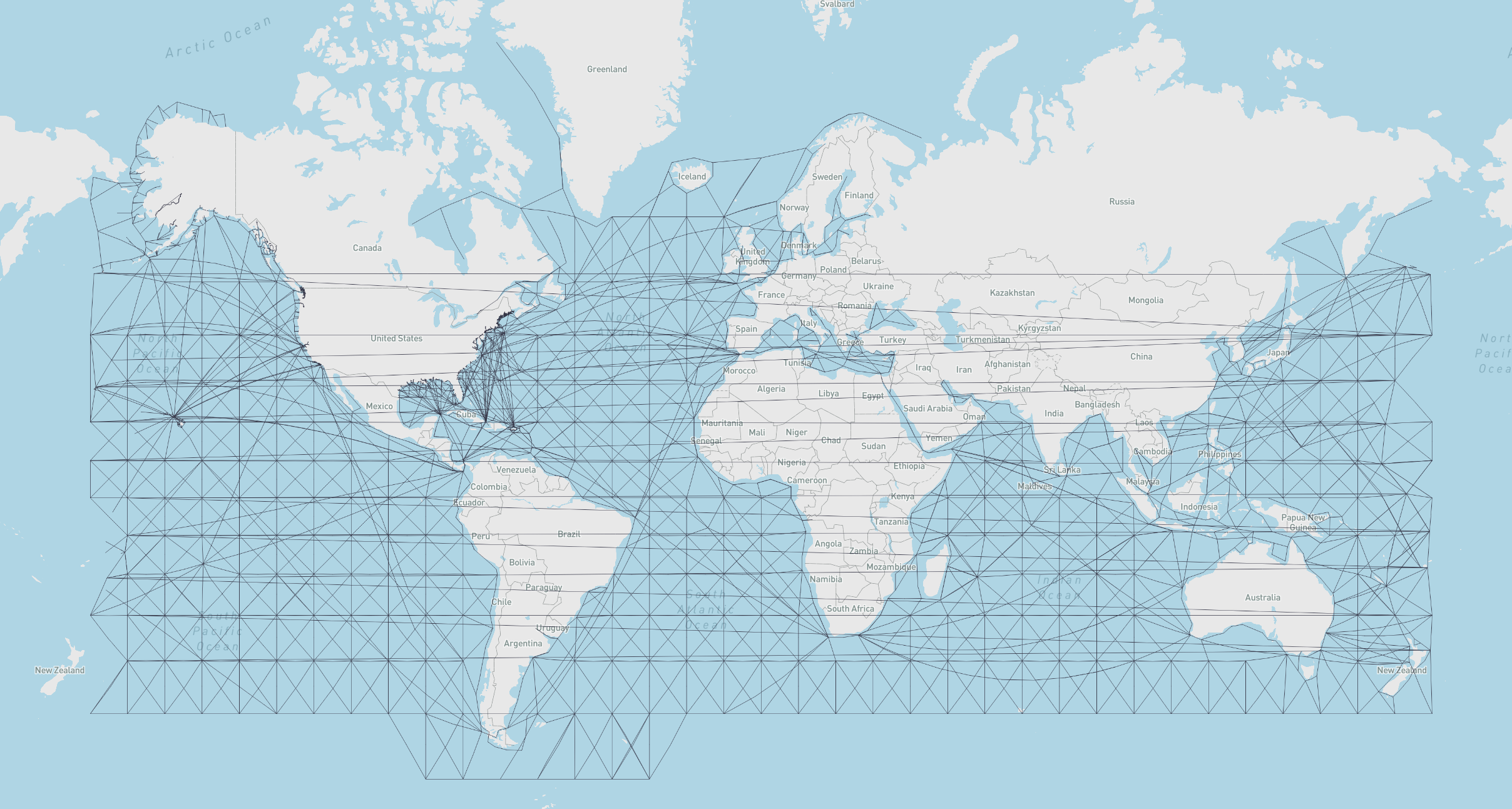
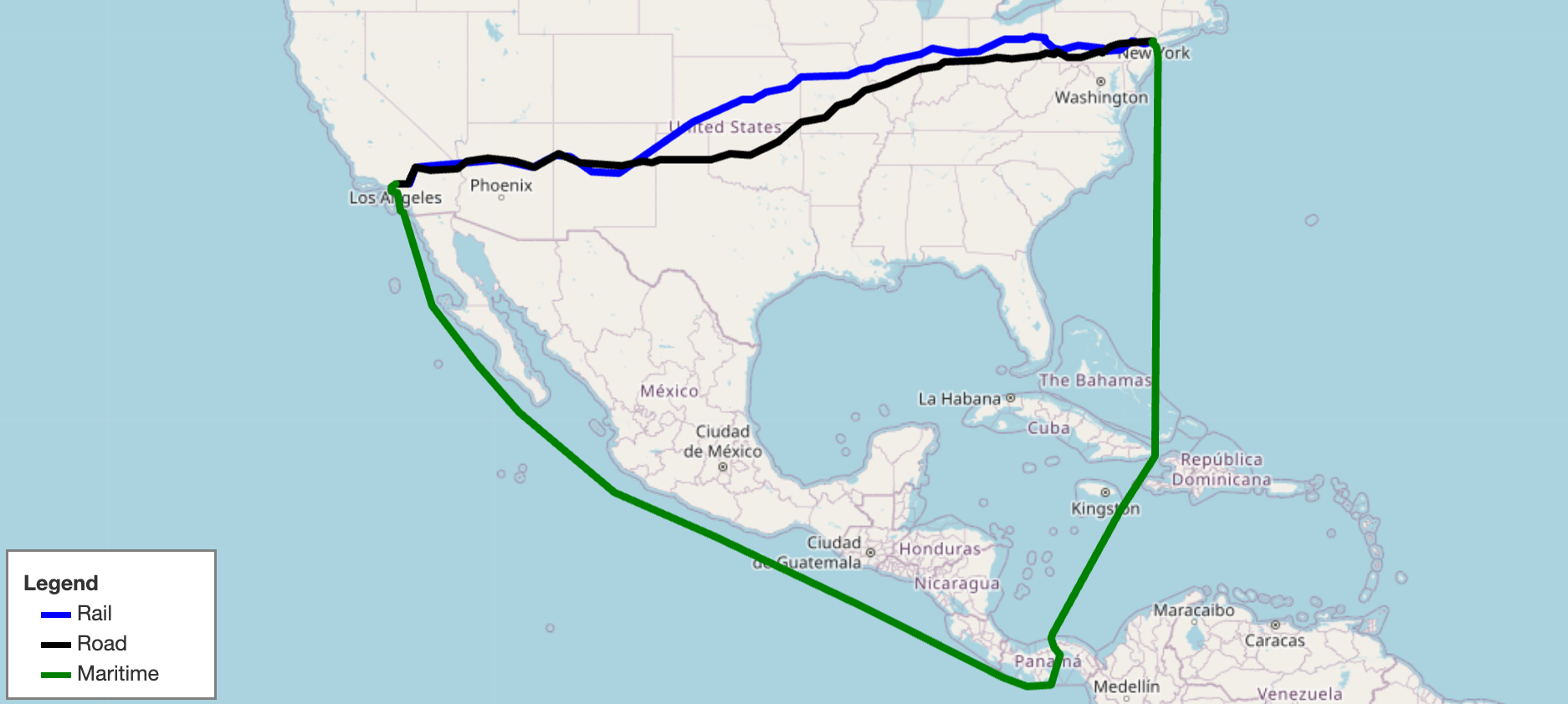
Supply chain graph package for Python

Documentation

Getting Started: https://github.com/connor-makowski/scgraph

Low Level: https://connor-makowski.github.io/scgraph/scgraph/core.html

Key Features

• Calculate the shortest path between two points on earth using a latitude / longitude pair
  • Inputs:
    • A latitude / longitude pair for the origin
    • A latitude / longitude pair for the destination
  • Calculation:
    • Algorithms:
      • Dijkstra's algorithm (Modified for sparse networks)
        • Modified to support sparse network data structures
      • Makowski's Modified Sparse Dijkstra algorithm
        • Modified for O(n) performance on particularly sparse networks
      • Possible future support for other algorithms
    • Distances:
      • Uses the haversine formula to calculate the distance between two points on earth
  • Returns:
    • path:
      • A list of dictionaries (latitude and longitude) that make up the shortest path
    • length:
      • The distance in kilometers between the two points
• Antimeridian support
• Arbitrary start and end points
• Arbitrary network data sets
• Grid based graphs
• Cached shortest path calculations for very fast repetative calculations to or from the same point in a graph.
  • Note: Geographs are not yet supported for this feature

Setup

Make sure you have Python 3.10.x (or higher) installed on your system. You can download it here.

Note: Support for python3.6-python3.9 is available up to version 2.2.0.

Installation

pip install scgraph

Use with Google Colab

• Getting Started
• Creating A Multi Path Geojson
• Modifying A Geograph

Getting Started

Basic Usage

Get the shortest path between two points on earth using a latitude / longitude pair In this case, calculate the shortest maritime path between Shanghai, China and Savannah, Georgia, USA.

# Use a maritime network geograph
from scgraph.geographs.marnet import marnet_geograph

# Get the shortest path between
output = marnet_geograph.get_shortest_path(
    origin_node={"latitude": 31.23,"longitude": 121.47},
    destination_node={"latitude": 32.08,"longitude": -81.09},
    output_units='km'
)
print('Length: ',output['length']) #=> Length:  19596.4653

In the above example, the output variable is a dictionary with three keys: length and coordinate_path.

• length: The distance between the passed origin and destination when traversing the graph along the shortest path
  • Notes:
    • This will be in the units specified by the output_units parameter.
    • output_units options:
      • km (kilometers - default)
      • m (meters)
      • mi (miles)
      • ft (feet)
• coordinate_path: A list of lists [latitude,longitude] that make up the shortest path

For more examples including viewing the output on a map, see the example notebook.

Included GeoGraphs

• marnet_geograph:
  • What: A maritime network data set from searoute
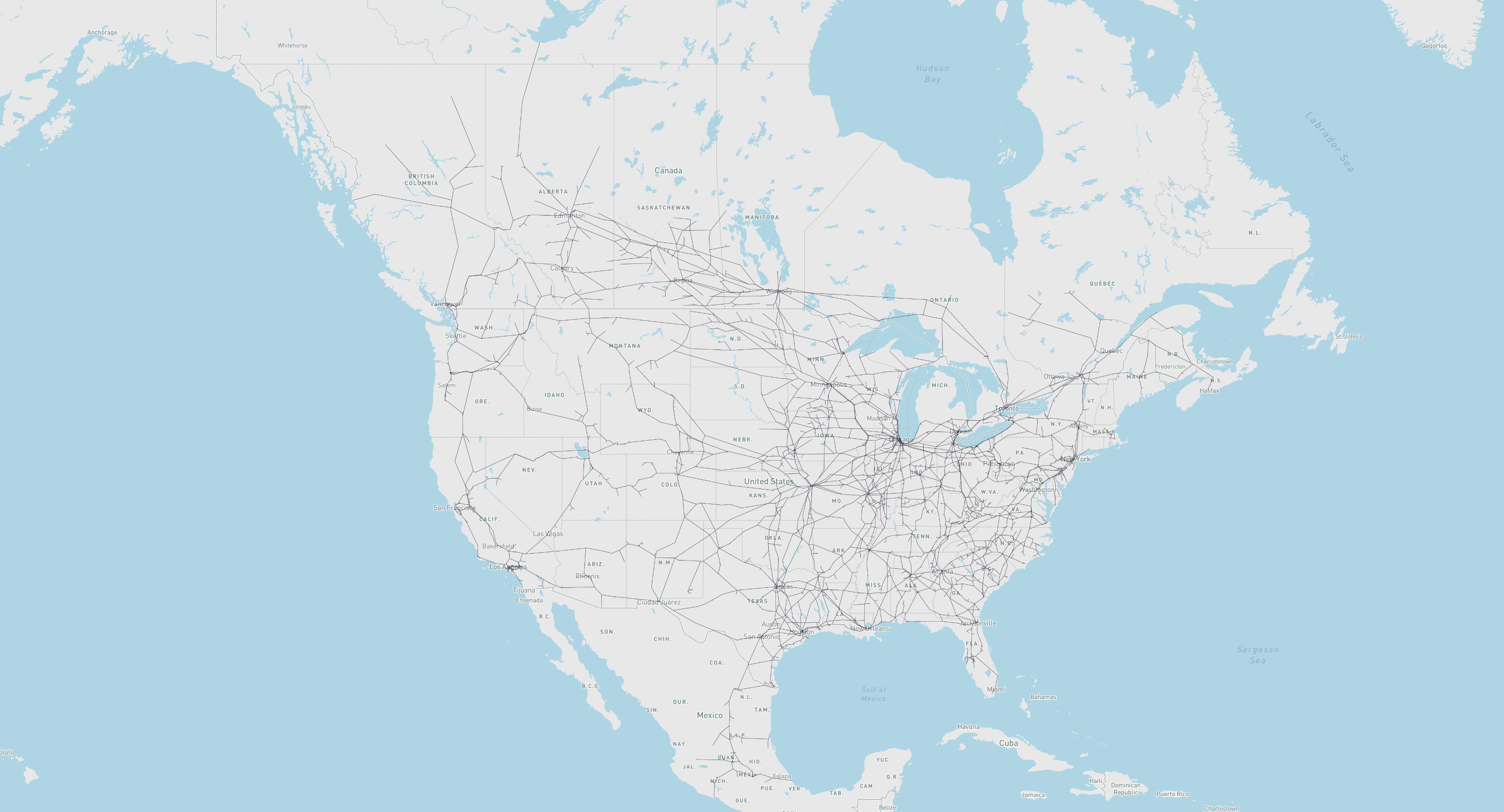
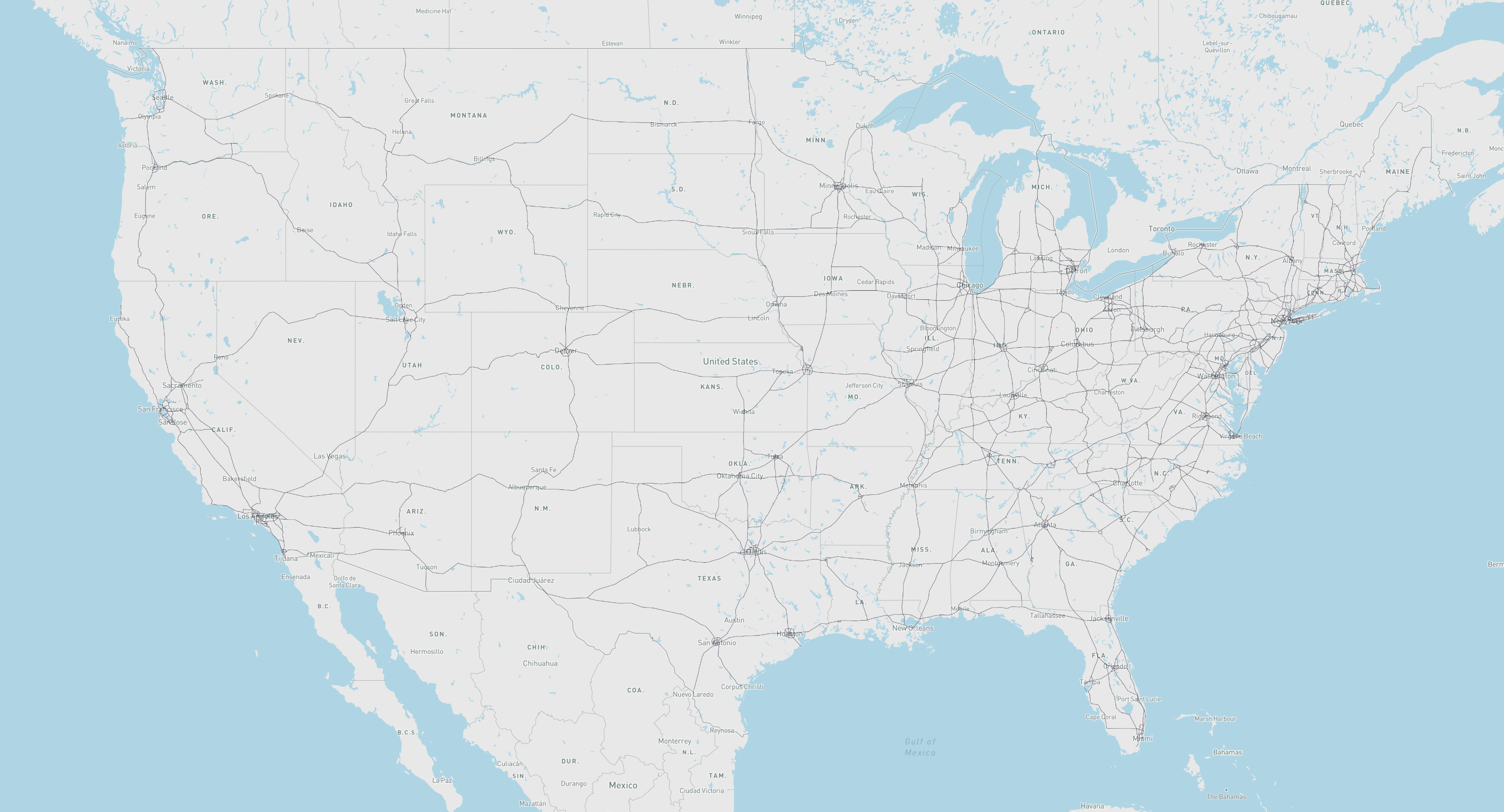
  • Use: from scgraph.geographs.marnet import marnet_geograph
  • Attribution: searoute
  • Length Measurement: Kilometers
  • Marnet Picture
• oak_ridge_maritime_geograph:
  • What: A maritime data set from the Oak Ridge National Laboratory campus
  • Use: from scgraph.geographs.oak_ridge_maritime import oak_ridge_maritime_geograph
  • Attribution: Oak Ridge National Laboratory with data from Geocommons
  • Length Measurement: Kilometers
  • Oak Ridge Maritime Picture
• north_america_rail_geograph:
  • What: Class 1 Rail network for North America
  • Use: from scgraph.geographs.north_america_rail import north_america_rail_geograph
  • Attribution: U.S. Department of Transportation: ArcGIS Online
  • Length Measurement: Kilometers
  • North America Rail Picture
• us_freeway_geograph:
  • What: Freeway network for the United States
  • Use: from scgraph.geographs.us_freeway import us_freeway_geograph
  • Attribution: U.S. Department of Transportation: ArcGIS Online
  • Length Measurement: Kilometers
  • US Freeway Picture
• scgraph_data geographs:
  • What: Additional geographs are available in the scgraph_data package
    • Note: These include larger geographs like the world highways geograph and world railways geograph.
  • Installation: pip install scgraph_data
  • Use: from scgraph_data.world_highways import world_highways_geograph
  • See: scgraph_data for more information and all available geographs.

GridGraph usage

Example:

• Create a grid of 20x100 cells.
  • This creates a grid based graph with connections to all 8 neighbors for each grid item.
  • Each grid item has 4 cardinal connections at length 1 and 4 diagonal connections at length sqrt(2)
• Create a wall from (10,5) to (10,99).
  • This would foce any path to go to the bottom of the graph to get around the wall.
• Get the shortest path between (2,10) and (18,10)
  • Note: The length of this path should be 16 without the wall and 20.9704 with the wall.

from scgraph import GridGraph

x_size = 20
y_size = 20
blocks = [(10, i) for i in range(5, y_size)]

# Create the GridGraph object
gridGraph = GridGraph(
    x_size=x_size,
    y_size=y_size,
    blocks=blocks,
    add_exterior_walls=True,
)

# Solve the shortest path between two points
output = gridGraph.get_shortest_path(
    origin_node={"x": 2, "y": 10},
    destination_node={"x": 18, "y": 10},
    # Optional: Specify the output coodinate format (default is 'list_of_dicts)
    output_coordinate_path="list_of_lists",
    # Optional: Cache the origin point spanning_tree for faster calculations on future calls
    cache=True,
    # Optional: Specify the node to cache the spanning tree for (default is the origin node)
    # Note: This first call will be slower, but future calls using this origin node will be substantially faster
    cache_for="origin",
)

print(output)
#=> {'length': 20.9704, 'coordinate_path': [[2, 10], [3, 9], [4, 8], [5, 8], [6, 7], [7, 6], [8, 5], [9, 4], [10, 4], [11, 4], [12, 5], [13, 6], [14, 7], [15, 7], [16, 8], [17, 9], [18, 10]]}

Advanced Usage

Using scgraph_data geographs:

• Note: Make sure to install the scgraph_data package before using these geographs

from scgraph_data.world_railways import world_railways_geograph

# Get the shortest path between Kalamazoo Michigan and Detroit Michigan by Train
output = world_railways_geograph.get_shortest_path(
    origin_node={"latitude": 42.29,"longitude": -85.58},
    destination_node={"latitude": 42.33,"longitude": -83.05}
)

Get a geojson line path of an output for easy visualization:

• Note: mapshaper.org and geojson.io are good tools for visualizing geojson files

from scgraph.geographs.marnet import marnet_geograph
from scgraph.utils import get_line_path

 # Get the shortest sea path between Sri Lanka and Somalia
output = marnet_geograph.get_shortest_path(
    origin_node={"latitude": 7.87,"longitude": 80.77},
    destination_node={"latitude": 5.15,"longitude": 46.20}
)
# Write the output to a geojson file
get_line_path(output, filename='output.geojson')

Modify an existing geograph: See the notebook here

You can specify your own custom graphs for direct access to the solving algorithms. This requires the use of the low level Graph class

from scgraph import Graph

# Define an arbitrary graph
# See the graph definitions here:
# https://connor-makowski.github.io/scgraph/scgraph/core.html#GeoGraph
graph = [
    {1: 5, 2: 1},
    {0: 5, 2: 2, 3: 1},
    {0: 1, 1: 2, 3: 4, 4: 8},
    {1: 1, 2: 4, 4: 3, 5: 6},
    {2: 8, 3: 3},
    {3: 6}
]

# Optional: Validate your graph
Graph.validate_graph(graph=graph)

# Get the shortest path between idx 0 and idx 5
output = Graph.dijkstra_makowski(graph=graph, origin_id=0, destination_id=5)
#=> {'path': [0, 2, 1, 3, 5], 'length': 10}

You can also use a slightly higher level GeoGraph class to work with latitude / longitude pairs

from scgraph import GeoGraph

# Define nodes
# See the nodes definitions here:
# https://connor-makowski.github.io/scgraph/scgraph/core.html#GeoGraph
nodes = [
    # London
    [51.5074, -0.1278],
    # Paris
    [48.8566, 2.3522],
    # Berlin
    [52.5200, 13.4050],
    # Rome
    [41.9028, 12.4964],
    # Madrid
    [40.4168, -3.7038],
    # Lisbon
    [38.7223, -9.1393]
]
# Define a graph
# See the graph definitions here:
# https://connor-makowski.github.io/scgraph/scgraph/core.html#GeoGraph
graph = [
    # From London
    {
        # To Paris
        1: 311,
    },
    # From Paris
    {
        # To London
        0: 311,
        # To Berlin
        2: 878,
        # To Rome
        3: 1439,
        # To Madrid
        4: 1053
    },
    # From Berlin
    {
        # To Paris
        1: 878,
        # To Rome
        3: 1181,
    },
    # From Rome
    {
        # To Paris
        1: 1439,
        # To Berlin
        2: 1181,
    },
    # From Madrid
    {
        # To Paris
        1: 1053,
        # To Lisbon
        5: 623
    },
    # From Lisbon
    {
        # To Madrid
        4: 623
    }
]

# Create a GeoGraph object
my_geograph = GeoGraph(nodes=nodes, graph=graph)

# Optional: Validate your graph
my_geograph.validate_graph()

# Optional: Validate your nodes
my_geograph.validate_nodes()

# Get the shortest path between two points
# In this case, Birmingham England and Zaragoza Spain
# Since Birmingham and Zaragoza are not in the graph,
# the algorithm will add them into the graph.
# See: https://connor-makowski.github.io/scgraph/scgraph/core.html#GeoGraph.get_shortest_path
# Expected output would be to go from
# Birmingham -> London -> Paris -> Madrid -> Zaragoza

output = my_geograph.get_shortest_path(
    # Birmingham England
    origin_node = {'latitude': 52.4862, 'longitude': -1.8904},
    # Zaragoza Spain
    destination_node = {'latitude': 41.6488, 'longitude': -0.8891}
)
print(output)
# {
#     'length': 1799.4323,
#     'coordinate_path': [
#         [52.4862, -1.8904],
#         [51.5074, -0.1278],
#         [48.8566, 2.3522],
#         [40.4168, -3.7038],
#         [41.6488, -0.8891]
#     ]
# }

Development

Running Tests, Prettifying Code, and Updating Docs

Make sure Docker is installed and running on a Unix system (Linux, MacOS, WSL2).

• Create a docker container and drop into a shell

  • ./run.sh

• Run all tests (see ./utils/test.sh)

  • ./run.sh test

• Prettify the code (see ./utils/prettify.sh)

  • ./run.sh prettify

• Update the docs (see ./utils/docs.sh)

  • ./run.sh docs

• Note: You can and should modify the Dockerfile to test different python versions.

Attributions and Thanks

Originally inspired by searoute including the use of one of their datasets that has been modified to work properly with this package.