Research
Security News
Kill Switch Hidden in npm Packages Typosquatting Chalk and Chokidar
Socket researchers found several malicious npm packages typosquatting Chalk and Chokidar, targeting Node.js developers with kill switches and data theft.
A high-performant C++ implementation of benchmark functions for mathematical optimization algorithms.
Benchmarkfcns is an effort to provide a high-perfomant, public and free implementation of well-known benchmark functions for mathematical optimization algorithms in Python. The Python library is implemented in C++ and utilizes powerful SIMD vector calucluations to offer very fast and efficient evaluation of the implemented functions on large batches of data.
For the documentation of the implemented functions and their features, please visit https://benchmarkfcns.info.
The library is packaged and available on the PyPI index. To install, simply run pip install benchmarkfcns.
After installing, using the library is straightforward and all that is needed is to import the needed functions, construct a matrix of input values and call the function. It should be noted that all the functions in the library only accept matrices as input. The rows of the matrix represent the data points at which the function should be evaluated and the columns represent the dimensions of data points. The code snippet shows how to use the library.
# Import the needed function.
from benchmarkfcns import rastrigin
import numpy as np

# Look at the function's documentation.
print(rastrigin.__doc__)

# The input matrix can be list of lists.
data = [[0, 0, 0]]

# Evaluate the Rastrigin function at (0, 0, 0).
results = rastrigin(data)
print(results)

# The input can also be a Numpy matrix.
data = np.array([[0, 0, 0], [1, 1, 1]])
results = rastrigin(data)
print(results)
This library is implemented to be as compatible as possible with all the mainstream plotting libraries. As a result, you are free to select your favourite plotting library to plot the functions in this library.
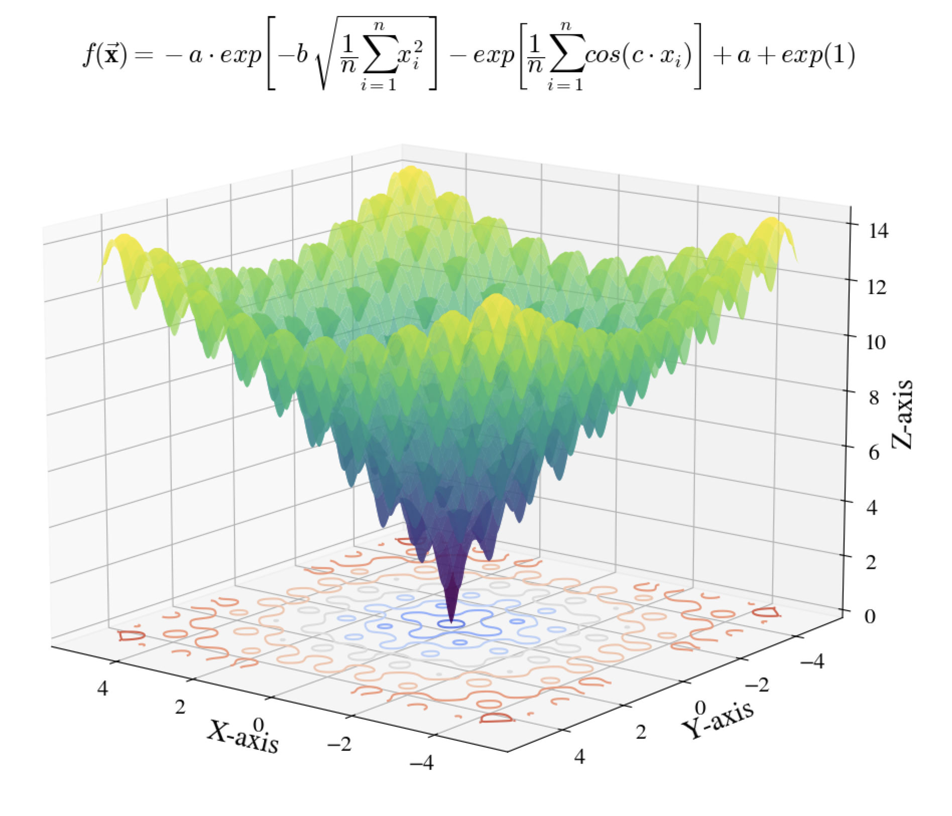
Plotting a mathematical function like rastrigin requires evaluating the function at a rather large set of data points. This is where the vectorized implementation of the functions in this package can shine as it allows performing the evaluations in a single function call, which significantly speeds up the plotting and reduces the computation cost. To facilitate this, the library also contains a helper function, meshgrid, for drawing 3D plots using the vectorized implemetations of the mathematical functions in this library. Given a list of x and y coordinates and a function, this function creates a meshgrid of points, evaluates the function over the meshgrid and returns the corresponding x, y and z points of the meshgrid that can be plotted with any plotting library.
from benchmarkfcns import ackley
from benchmarkfcns.plotting import meshgrid

# Using the matplotlib library for this example
import matplotlib.pyplot as plt
import numpy as np

# Used to make title equation look nicer
import matplotlib
matplotlib.rcParams['mathtext.fontset'] = 'cm'
matplotlib.rcParams['font.family'] = 'STIXGeneral'

# We want to plot the function for x and y in range [-5, 5].
# This corresponds to a grid of 100,000,000 points.
x = np.linspace(-5, 5, 10000)
y = np.linspace(-5, 5, 10000)

# `meshgrid` creates the 3D meshgrid and evaluates `ackley` on it.
# Evaluation of 100,000,000 points took less than 3 seconds.
X, Y, Z = meshgrid(x, y, ackley)

# Create the plot
fig = plt.figure()
ax = fig.add_subplot(111, projection='3d')

# Plot the surface and its contour with a colormap
ax.plot_surface(X, Y, Z, cmap='viridis', alpha=0.7)
ax.contour(X, Y, Z, zdir='z', offset=0, cmap='coolwarm')

# Set labels and title
ax.set_xlabel('X-axis')
ax.set_ylabel('Y-axis')
ax.set_zlabel('Z-axis')
plt.suptitle(r"$f({\bf \vec{x}}) = -a\cdot exp\left[-b\,\sqrt{\dfrac{1}{n}\sum_{i=1}^{n}x_{i}^{2}}\right]-exp\left[\dfrac{1}{n}\sum_{i=1}^{n}cos(c\cdot x_{i})\right]+ a + exp(1)$")

# Set view angle and display
ax.view_init(14, 120)
plt.show()

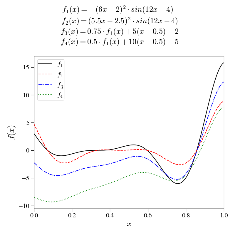
Addition of multi-fidelity functions such as the forrester function, shown below.
import benchmarkfcns.multifidelity as mfb

# Using the matplotlib library for this example
import matplotlib.pyplot as plt
import numpy as np

# Used to make title equation look nicer
import matplotlib
matplotlib.rcParams['mathtext.fontset'] = 'cm'
matplotlib.rcParams['font.family'] = 'STIXGeneral'

# We want to plot the function for x in range [0, 1].
x = np.linspace(0, 1, 10000)

# Evaluation of points took less than 340 \mu\,s, per function.
f = mfb.forrester(x)

# Create the plot
fig = plt.figure(figsize=(8,8))
ax = fig.add_subplot(111)

# Plot all 4 fidelity levels.
ax.plot(x, f[:, 0], 'k-', label=r"$f_{1}$")
ax.plot(x, f[:, 1], 'r--', label=r"$f_{2}$")
ax.plot(x, f[:, 2], 'b-.', label=r"$f_{3}$")
ax.plot(x, f[:, 3], 'g:', label=r"$f_{4}$")

# Add labels, limits, and legend.
ax.set_xlabel(r"$x$")
ax.set_ylabel(r"$f(x)$")
ax.set_xlim(0,1)
ax.set_ylim(-10.5,17)

plt.suptitle(
    r"$f_{1}(x) =~~~(6x - 2)^{2} \cdot sin(12x - 4)$"
    + f"\n"
    + r"$~~f_{2}(x) = (5.5x - 2.5)^{2} \cdot sin(12x - 4)$"
    + f"\n"
    + r"$~~f_{3}(x) = 0.75 \cdot f_{1}(x) + 5(x - 0.5) - 2$"
    + f"\n"
    + r"$~~f_{4}(x) = 0.5 \cdot f_{1}(x) + 10(x - 0.5) - 5$"
    )

plt.legend()
plt.tight_layout()
plt.show()

As a reference, the repository also contains the implementation of the functions in MATLAB. To install and use the MATLAB implementation, it is just required to add the project folders to MATLAB's path. For example, to use the functions in the 'benchmarks/MATLAB' folder, just navigate to this folder with MATLAB's directory explorer or use the command addpath with path to the folder on your PC (e.g. addpath /path/to/benchmarks).
The library is built with the pybind11, scikit-build-core and Eigen libraries. To compile the library, you will need to have CMake version 3.15 or above installed and configured. The easiest way to compile and install the package locally is to clone the repository into a directory, e.g. BenchmarkFcns, with submodules initialized using git submodule update --init --recursive, and then run pip install ./BenchmarkFcns. Although optional, it is highly recommended to install the package into a virtual environment.
Any suggestions and contributions are welcomed. The best way to contribute to the library is to fork the repository, apply the contributions and create a pull request.
Any bug reports, code contributions, suggestions, feedback and insights are greatly appreciated. If you are using this library in a research publication, please kindly consider citing the repository using the following:
For the general reference of the repository:
Mazhar Ansari Ardeh and cmutnik. (2024). Benchmarkfcns. Zenodo. https://doi.org/10.5281/zenodo.14556621
For the latest version of the repository (v3.0.0):
Mazhar Ansari Ardeh and cmutnik. (2024). Benchmarkfcns (bersion v3.0.0). Zenodo. https://doi.org/10.5281/zenodo.14556622
FAQs
A high-performant C++ implementation of benchmark functions for mathematical optimization algorithms.
We found that benchmarkfcns demonstrated a healthy version release cadence and project activity because the last version was released less than a year ago. It has 1 open source maintainer collaborating on the project.
Did you know?

Socket for GitHub automatically highlights issues in each pull request and monitors the health of all your open source dependencies. Discover the contents of your packages and block harmful activity before you install or update your dependencies.

Research
Security News
Socket researchers found several malicious npm packages typosquatting Chalk and Chokidar, targeting Node.js developers with kill switches and data theft.

Security News
pnpm 10 blocks lifecycle scripts by default to improve security, addressing supply chain attack risks but sparking debate over compatibility and workflow changes.

Product
Socket now supports uv.lock files to ensure consistent, secure dependency resolution for Python projects and enhance supply chain security.