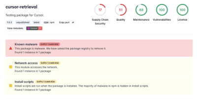
Security News
The Risks of Misguided Research in Supply Chain Security
Snyk's use of malicious npm packages for research raises ethical concerns, highlighting risks in public deployment, data exfiltration, and unauthorized testing.
JijModeling is a Python package designed to intuitively write mathematical optimization models. Its main features are:
JijModeling is a tool for writing models using Python code, it does not evaluate or solve the models. The main motivation is to focus on the algebraic structure of the models, so that they can be reasoned about, verified and more nimbly altered regardless of the instance data, while still serving as a step towards generating the input formats the solvers expect.
To be used with solvers, it needs to be paired with the actual instance data and converted into the specific solver’s input format by another tool, such as our internal JijZept services, or with the freely available jijmodeling-transpiler.
If you use pip, you can install JijModeling with:
pip install jijmodeling
Note that JijModeling requires Python 3.9 or higher.
To get a better idea of how to use jijmodeling, we’ll go over a basic example, starting with writing a simple model, converting it, then executing it with a solver. For the first two sections, jijmodeling is all you need, but we recommend using a Jupyter notebook to easily check LaTeX output.
For the third section, we will be using JijModelingTranspiler and OpenJij. Note that jijmodeling models are also usable with our paid JijZept services. JijMdelingTranspiler and OpenJij can be installed as usual through pip:
pip install jijmodeling-transpiler openjij
Working with JijModeling should feel natural to anyone familiar with mathematical optimization models.
We represent various mathematical expressions by combining various classes, like BinaryVar and Placeholder using basic mathematical operations. ___Var classes refer to different kinds of decision variables. Placeholder represents just about any kind of constant or value to be specified later. That is, they’re something we want to abstract away from the model and mark as part of instance-specific data. You can also use number literals, of course.
import jijmodeling as jm

x = jm.BinaryVar("x")
y = jm.IntegerVar("y", lower_bound=1, upper_bound=10)
n = jm.Placeholder("n")
exp = x * (y ** 2) * n
The placeholder and variables above are zero-dimensional (scalars), but we can also represent arrays/multi-dimensional variables and constants using these classes, as we’ll see later on.
In JijModeling, we build up a model by adding expressions like this to a Problem object, representing our model as a whole. Constraints are defined by the Constraint class wrapping around some comparison expression. (Note that only <=, ==, and >= are supported in Constraints).
a = jm.IntegerVar("a", lower_bound=5, upper_bound=20)
b = jm.IntegerVar("b", lower_bound=1, upper_bound=20)
c = jm.IntegerVar("c", lower_bound=20, upper_bound=30)
n = jm.Placeholder("n")

problem = jm.Problem("my problem")
problem += n * (a + b + c)
problem += jm.Constraint("c1", 2 * (b + c) <= 75)
problem += jm.Constraint("c2", a + b <= 40)
problem
The above should output a model like this: (in a Jupyter notebook you’ll also see a description of the decision variables, omitted here for brevity)
$$ \begin{array}{cccc}\text{Problem:} & \text{my problem} & & \ & & \min \quad \displaystyle n \cdot \left(a + b + c\right) & \ \text{{s.t.}} & & & \ & \text{c1} & \displaystyle 2 \cdot \left(b + c\right) \leq 75 & \ & \text{c2} & \displaystyle a + b \leq 40 \ \end{array} $$
Let’s see how we would model a generic Knapsack problem.
In this problem, we have $N$ valuable items. We want to take as many items as possible, but we can only carry so much with us, determined by a weight limit $W$. We’ll be representing the decision to take some item $i$ with the binary variable $x_{i}$. That item’s weight is $w_i$ and its value $v_i$.
Let’s first define these values:
W = jm.Placeholder("W") # The maximum weight we can carry
# The values and weights of each items can represented as
# one-dimensional Placeholders.
values = jm.Placeholder("v", ndim=1)
weights = jm.Placeholder("w", ndim=1)
# We can define N in relation to the size of our placeholders,
# so it's calculated automatically based on the instance data.
# The optional "latex" parameter lets us define how this is
# displayed in the LaTeX output.
N = values.len_at(0, latex="N")

# we have N decision variables, which we represent with a
# one-dimensional BinaryVar. We must specify that it has N elements.
x = jm.BinaryVar("x", shape=(N,))

# an index we'll use for summations
i = jm.Element("i", (0,N))
At the end we create an Element. These are used as indices. With jijmodeling.sum, this allows us to write summations in a style similar to Sigma notation. Here we define that this index goes from 0 (inclusive) to $N$ (non-inclusive). It can feel strange to write these ahead of time, but doing so allows us to reuse it and is more convenient overall.
For this problem we want to maximize our total value, while making sure the total weight is within our limit. We can write that like this:
problem = jm.Problem("knapsack", sense = jm.ProblemSense.MAXIMIZE)
problem += jm.sum(i, values[i] * x[i])
problem += jm.Constraint("weight limit", jm.sum(i, weights[i] * x[i]) <= W)
problem
This gives us the model we’d expect:
$$ \begin{array}{cccc}\text{Problem:} & \text{knapsack} & & \ & & \max \quad \displaystyle \sum_{i = 0}^{N - 1} v_{i} \cdot x_{i} & \ \text{{s.t.}} & & & \ & \text{weight limit} & \displaystyle \sum_{i = 0}^{N - 1} w_{i} \cdot x_{i} \leq W & \ \text{{where}} & & & \ & x & 1\text{-dim binary variable}\ \end{array} $$
As a reminder, JijModeling expressions can be stored in variables like regular python objects. When working with larger problems, complex expressions can be built up from smaller ones, which can be easier to understand and modify later. For a problem this small this is not that useful, but just to illustrate, the previous code snippet could be rewritten like this:
chosen_v = values[i] * x[i]
chosen_w = weights[i] * x[i]
sum_of_values = jm.sum(i, chosen_v)
sum_of_weights = jm.sum(i, chosen_w)
weight_below_limit = sum_of_weights <= W

problem = jm.Problem("knapsack", sense = jm.ProblemSense.MAXIMIZE)
problem += sum_of_values
problem += jm.Constraint("weight limit", weight_below_limit)
problem
These two models are equivalent. How you write the model is a matter of preference and convenience.
Now we have our model, though not much can be done with it by itself other than exporting it to LaTeX. We can pair it with instance data to generate the input for an optimization solver. To demonstrate, let’s see how we’d use it with the freely available JijModelingTranspiler to convert it, and OpenJij to solve the model. Note that our tooling provided with JijZept also accepts JijModeling models as input.
This is meant as a quick demonstration, not a full introduction to JijModelingTranspiler and OpenJij features. You can check their documentation for more information.
With JijModelingTranspiler, we can pass along our instance data to create an intermediary representation that can be converted to different formats quickly, but in our case we'll just convert it to QUBO.
from jijmodeling_transpiler.core import compile_model
from jijmodeling_transpiler.core.pubo import transpile_to_pubo

data = {
 "W": 100,
 "v": [100, 90, 80, 70, 60, 50, 40, 30],
 "w": [1, 5, 10, 20, 30, 40, 50, 60, 70],
}

compiled = compile_model(problem, data)
qubo, _ = transpile_to_pubo(compiled).get_qubo_dict()
qubo
We now have a QUBO dictionary, which is valid input for certain optimization solvers. Writing out this kind of dictionary by hand would be very prone to error, but thankfully we just had to write out the model in a human-friendly way which is easier to verify. We can now use this dictionary with openjij to actually solve the problem:
import openjij as oj

sampler = oj.SASampler()
response = sampler.sample_qubo(qubo, num_reads=1)
response.first
This is using openjij's simulated annealing sampler, with the num_reads parameter saying we want to just sample it once. We can increase that to sample the solver multiple times, and then the response object would allow us to explore the different results. But for a problem of this size, all samples will just reach the optimal solution anyway, so here we’ve done a single sample and are looking at just the “best” solution found. It’s an object that looks like:
Sample(sample={0: 1, 1: 1, 2: 1, 3: 1, 4: 1, 5: 1, 6: 0, 7: 0}, energy=-5.501111111111113, num_occurrences=1)
The sample dictionary gives us the value the solver figured out for each of the decision variables. There’s a lot more that can be done here with Transpiler and OpenJij to better process and visualize the results, or reuse the same model for different purposes, but for that you should check out their respective documentation pages.
FAQs
Mathematical modeling tool for optimization problem
We found that jijmodeling demonstrated a healthy version release cadence and project activity because the last version was released less than a year ago. It has 1 open source maintainer collaborating on the project.
Did you know?

Socket for GitHub automatically highlights issues in each pull request and monitors the health of all your open source dependencies. Discover the contents of your packages and block harmful activity before you install or update your dependencies.

Security News
Snyk's use of malicious npm packages for research raises ethical concerns, highlighting risks in public deployment, data exfiltration, and unauthorized testing.

Research
Security News
Socket researchers found several malicious npm packages typosquatting Chalk and Chokidar, targeting Node.js developers with kill switches and data theft.

Security News
pnpm 10 blocks lifecycle scripts by default to improve security, addressing supply chain attack risks but sparking debate over compatibility and workflow changes.