mixscatter

mixscatter

Table of Contents

• Overview
• Installation
• Documentation
• Example Showcase
• Contributing
• License

Overview

mixscatter is a pure python package for the calculation of scattering functions of multi-component mixtures of interacting spherical scatterers in the Born approximation (Rayleigh-Gans-Debye scattering).

Key Features:

• Calculation of scattering amplitudes, measurable intensities, form factors, structure factors, and diffusion coefficients.
• Flexible construction of systems with arbitrary compositions and complex scattering length density profiles.
• Suitable for researchers and developers working on particulate systems characterization.

Take a look at these publications if you are interested:

• P. Salgi and R. Rajagopalan, "Polydispersity in colloids: implications to static structure and scattering", Adv. Colloid Interface Sci. 43, 169-288 (1993)
• A. Vrij, "Mixtures of hard spheres in the Percus–Yevick approximation. Light scattering at finite angles", J. Chem. Phys. 71, 3267-3270 (1979)
• R. Botet, S. Kwok and B. Cabane, "Percus-Yevick structure factors made simple", J. Appl. Cryst. 53, 1570-1582 (2020)
• J. Diaz Maier, K. Gaus and J. Wagner, "Measurable structure factors of dense dispersions containing polydisperse, optically inhomogeneous particles", arXiv:2404.03470 [cond-mat.soft]

Installation

mixscatter is available on the Python Package Index (PyPI).

Prerequisites

Ensure you have Python 3.10 or higher installed.

Using pip

Install the package via pip:

pip install mixscatter

The source code is currently hosted on GitHub at: https://github.com/joelmaier/mixscatter

Documentation

Find the documentation on GitHub Pages: https://joelmaier.github.io/mixscatter/

Example Showcase

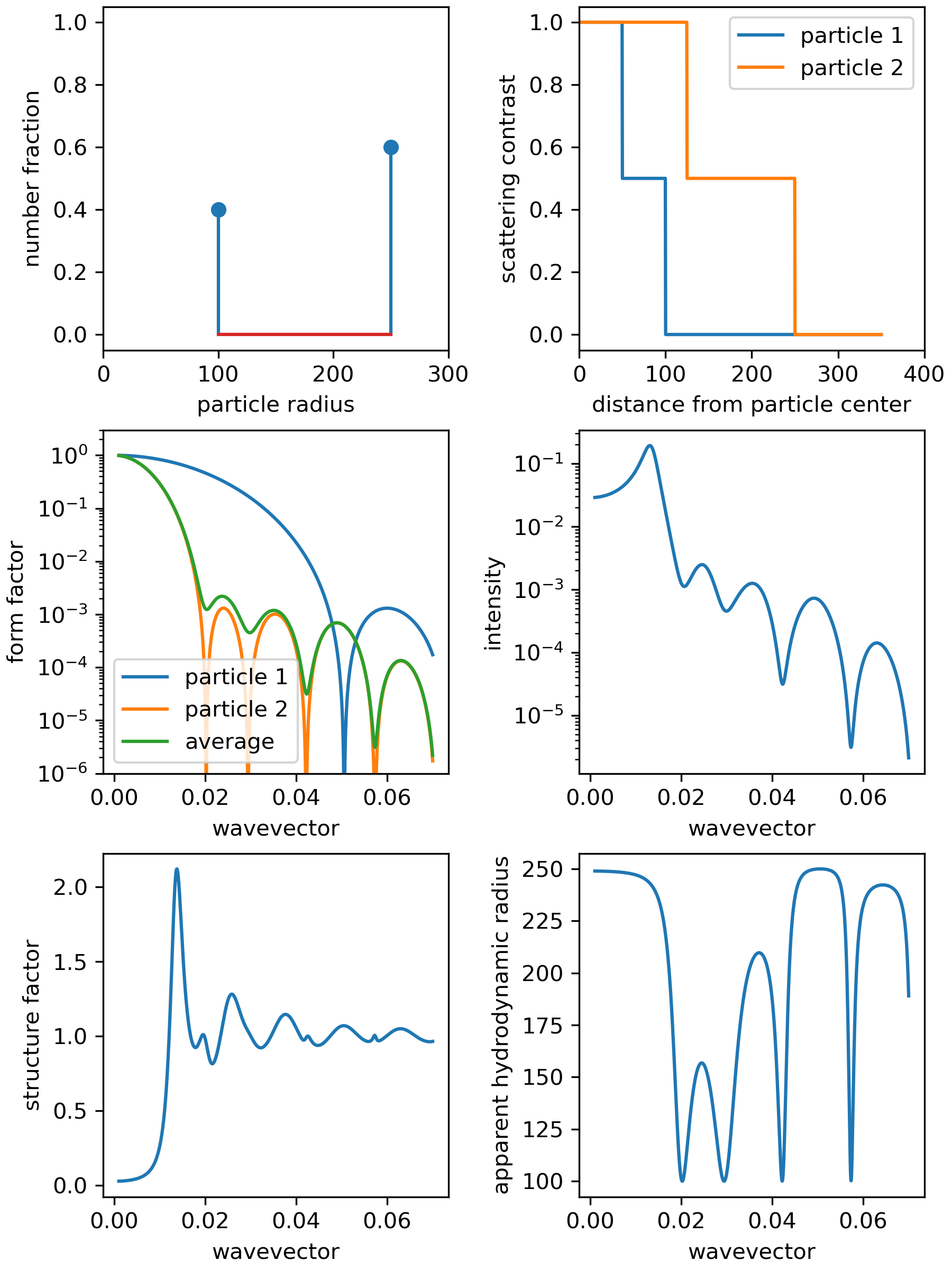
This example demonstrates the fundamental capabilities of mixscatter. For a comprehensive walk-through, refer to the Getting Started Guide.

Run this code to produce the figure below.

import numpy as np
import matplotlib.pyplot as plt

from mixscatter.mixture import Mixture
from mixscatter.scatteringmodel import SimpleCoreShell
from mixscatter.liquidstructure import PercusYevick
from mixscatter import (
    measurable_intensity,
    measurable_structure_factor,
    measurable_diffusion_coefficient
)

if __name__ == "__main__":
    plt.ion()
    plt.close("all")
    fig, ax = plt.subplots(3, 2, figsize=(6, 8), layout="constrained")

    # Initialize a particle mixture
    mixture = Mixture(radius=[100, 250], number_fraction=[0.4, 0.6])

    # Visualize mixture composition
    ax[0, 0].stem(mixture.radius, mixture.number_fraction)
    ax[0, 0].set_xlim(0, 300)
    ax[0, 0].set_ylim(-0.05, 1.05)
    ax[0, 0].set_xlabel("particle radius")
    ax[0, 0].set_ylabel("number fraction")

    # Provide a model for the optical properties of the system
    wavevector = np.linspace(1e-3, 7e-2, 1000)
    scattering_model = SimpleCoreShell(
        wavevector=wavevector,
        mixture=mixture,
        core_to_total_ratio=0.5,
        core_contrast=1.0,
        shell_contrast=0.5
    )

    # Visualize SLD profile
    distance = np.linspace(0, 350, 1000)
    for i, particle in enumerate(scattering_model.particles):
        profile = particle.get_profile(distance)
        ax[0, 1].plot(distance, profile, label=f"particle {i + 1}")
    ax[0, 1].set_xlim(0, 400)
    ax[0, 1].set_xlabel("distance from particle center")
    ax[0, 1].set_ylabel("scattering contrast")
    ax[0, 1].legend()

    # Visualize individual and average form factor(s)
    for i, form_factor in enumerate(scattering_model.single_form_factor):
        ax[1, 0].plot(wavevector, form_factor, label=f"particle {i + 1}")
    ax[1, 0].plot(
        wavevector, scattering_model.average_form_factor, label="average"
    )
    ax[1, 0].set_yscale("log")
    ax[1, 0].set_ylim(1e-6, 3e0)
    ax[1, 0].legend()
    ax[1, 0].set_xlabel("wavevector")
    ax[1, 0].set_ylabel("form factor")

    # Provide a model for the liquid structure
    liquid_structure = PercusYevick(
        wavevector=wavevector, mixture=mixture, volume_fraction_total=0.45
    )

    # Calculate the scattered intensity of the system
    intensity = measurable_intensity(liquid_structure, scattering_model)
    ax[1, 1].plot(wavevector, intensity)
    ax[1, 1].set_yscale("log")
    ax[1, 1].set_xlabel("wavevector")
    ax[1, 1].set_ylabel("intensity")

    # Calculate the experimentally obtainable, measurable structure factor
    structure_factor = measurable_structure_factor(
        liquid_structure, scattering_model
    )
    ax[2, 0].plot(wavevector, structure_factor)
    ax[2, 0].set_xlabel("wavevector")
    ax[2, 0].set_ylabel("structure factor")

    # Calculate the effective Stokes-Einstein diffusion coefficient
    # which would be obtained from a cumulant analysis in
    # dynamic light scattering
    diffusion_coefficient = measurable_diffusion_coefficient(
        scattering_model, thermal_energy=1.0, viscosity=1.0 / (6.0 * np.pi)
    )
    # Visualize the apparent hydrodynamic radius, which is
    # proportional to 1/diffusion_coefficient
    ax[2, 1].plot(wavevector, 1 / diffusion_coefficient)
    ax[2, 1].set_xlabel("wavevector")
    ax[2, 1].set_ylabel("apparent hydrodynamic radius")

    fig.savefig("simple_example_figure.png", dpi=300)

Contributing

Contributions are welcome! If you find any bugs or want to request features, feel free to get in touch or create an issue.

License

This project is licensed under the MIT License - see the LICENSE file for details.